An application of LMM in studying plant phenotypic plasticity.
The full tutorial and used datasets are acquired from this paper
key terms
- Phenotype, traits of an organism resulting from both genetic and environmental influences.
- Phenotypic plasticity, the ability of a single genotype to express different phenotypes under different environmental conditions.
- A reaction norm, describes the shape or specific form of the phenotypic response to the environment of an individual or genotype
Typical models of phenotypic plasticity

Figure1: Typical nonlinear reaction norm examples demonstrating the variety of shapes of plasticity in response to growth temperature (Figure source: https://nph.onlinelibrary.wiley.com/cms/asset/b09ccb52-7cad-4c8d-b1a5-472d027d07df/nph15656-fig-0001-m.jpg)
One thing to be noted for this Fig.1 is, if you only have two data points, there is no chance of recovering nonlinear norms.
 On Fig.2, each column represents one common basis function for non-linear reaction norm.
Different colored curves show different genotypes.
On Fig.2, each column represents one common basis function for non-linear reaction norm.
Different colored curves show different genotypes.
code practice
The original full dataset and code tutorial were downloaded from website as Supplementary File 3 and 4.
load data
##   genotype relativedate temperature ID
## 1        1     1.104052    5.000000  1
## 2        1     1.063095    6.666667  2
## 3        1    -1.226558    8.333333  3
## 4        1    -3.162186   10.000000  4
## 5        1    -2.516623   11.666667  5
## 6        1    -2.849256   13.333333  6
## 'data.frame': 200 obs. of 4 variables:
## $ genotype : int 1 1 1 1 1 1 1 1 1 1 ...
## $ relativedate: num 1.1 1.06 -1.23 -3.16 -2.52 ...
## $ temperature : num 5 6.67 8.33 10 11.67 ...
## $ ID : int 1 2 3 4 5 6 7 8 9 10 ...## 'data.frame': 200 obs. of 5 variables:
## $ genotype : Factor w/ 20 levels "1","2","3","4",..: 1 1 1 1 1 1 1 1 1 1 ...
## $ relativedate: num 1.1 1.06 -1.23 -3.16 -2.52 ...
## $ temperature : num 5 6.67 8.33 10 11.67 ...
## $ ID : int 1 2 3 4 5 6 7 8 9 10 ...
## $ loc : Factor w/ 10 levels "5","6.666666667",..: 1 2 3 4 5 6 7 8 9 10 ...## genotype relativedate temperature ID loc ctemperature
## 1 1 1.104052 5.000000 1 5 -1.5627772
## 2 1 1.063095 6.666667 2 6.666666667 -1.2154934
## 3 1 -1.226558 8.333333 3 8.333333333 -0.8682096
## 4 1 -3.162186 10.000000 4 10 -0.5209257
## 5 1 -2.516623 11.666667 5 11.66666667 -0.1736419
## 6 1 -2.849256 13.333333 6 13.33333333 0.1736419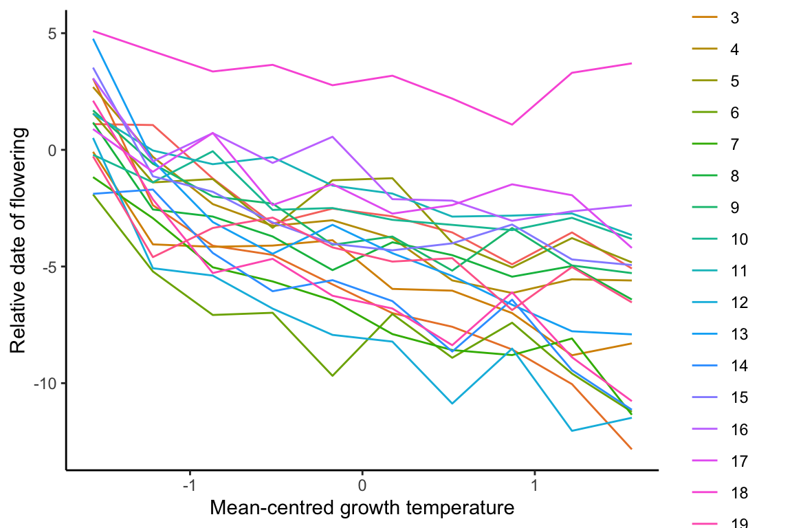
As mean-centred temperature (ctemperature) is the predictor, it is plotted on the x-axis.
An observation from this figure is, with increasing ctemperature, the variance among the genotypes also appear to increase.
building linear mixed model
- Treating different genotypes within the same location as
replicates. - In this case, the 20 genotypes, i.e., 20 observations, in location 1 are replicates within loc1, and contain information about within location variance.
- In linear mixed model, random effect contribute to variance, i.e., different locations may have different variance (estimated from variance among replicates). As in the very first figure, high temperature location tend to have larger variance.
## Linear mixed model fit by maximum likelihood  ['lmerMod']
## Formula: relativedate ~ ctemperature + (1 | loc)
##    Data: flowerdata
##
##      AIC      BIC   logLik deviance df.resid
##    998.2   1011.4   -495.1    990.2      196
##
## Scaled residuals:
##     Min      1Q  Median      3Q     Max
## -2.1925 -0.6741  0.0005  0.6485  3.7194
##
## Random effects:
##  Groups   Name        Variance Std.Dev.
##  loc      (Intercept) 0.1062   0.3259
##  Residual             8.1796   2.8600
## Number of obs: 200, groups:  loc, 10
##
## Fixed effects:
##              Estimate Std. Error t value
## (Intercept)   -3.6897     0.2270 -16.255
## ctemperature  -2.1124     0.2276  -9.283
##
## Correlation of Fixed Effects:
##             (Intr)
## ctemperatur 0.000
## R2m R2c
## [1,] 0.3500338 0.3583672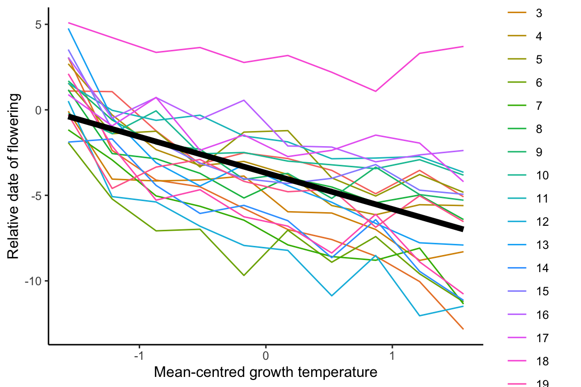
The plot helps us view how well the linear model fits the raw data by overlaying the regression line from model as an average population-level reaction norm.
R^2 value from the above linear mixed model is 0.36, which can be used to compare models built below.
building quadratic fixed effects model
## Linear mixed model fit by maximum likelihood  ['lmerMod']
## Formula: relativedate ~ poly(ctemperature, 2, raw = T) + (1 | loc)
##    Data: flowerdata
##
##      AIC      BIC   logLik deviance df.resid
##    993.9   1010.4   -492.0    983.9      195
##
## Scaled residuals:
##     Min      1Q  Median      3Q     Max
## -2.3650 -0.6812  0.0104  0.6009  3.4764
##
## Random effects:
##  Groups   Name        Variance Std.Dev.
##  loc      (Intercept) 0.000    0.000
##  Residual             8.019    2.832
## Number of obs: 200, groups:  loc, 10
##
## Fixed effects:
##                                 Estimate Std. Error t value
## (Intercept)                      -4.2757     0.3030 -14.113
## poly(ctemperature, 2, raw = T)1  -2.1124     0.2007 -10.523
## poly(ctemperature, 2, raw = T)2   0.5890     0.2285   2.578
##
## Correlation of Fixed Effects:
##             (Intr) p(,2,r=T)1
## pl(,2,r=T)1  0.000
## pl(,2,r=T)2 -0.750  0.000
## optimizer (nloptwrap) convergence code: 0 (OK)
## boundary (singular) fit: see help('isSingular')
## R2m R2c
## [1,] 0.3710001 0.3710001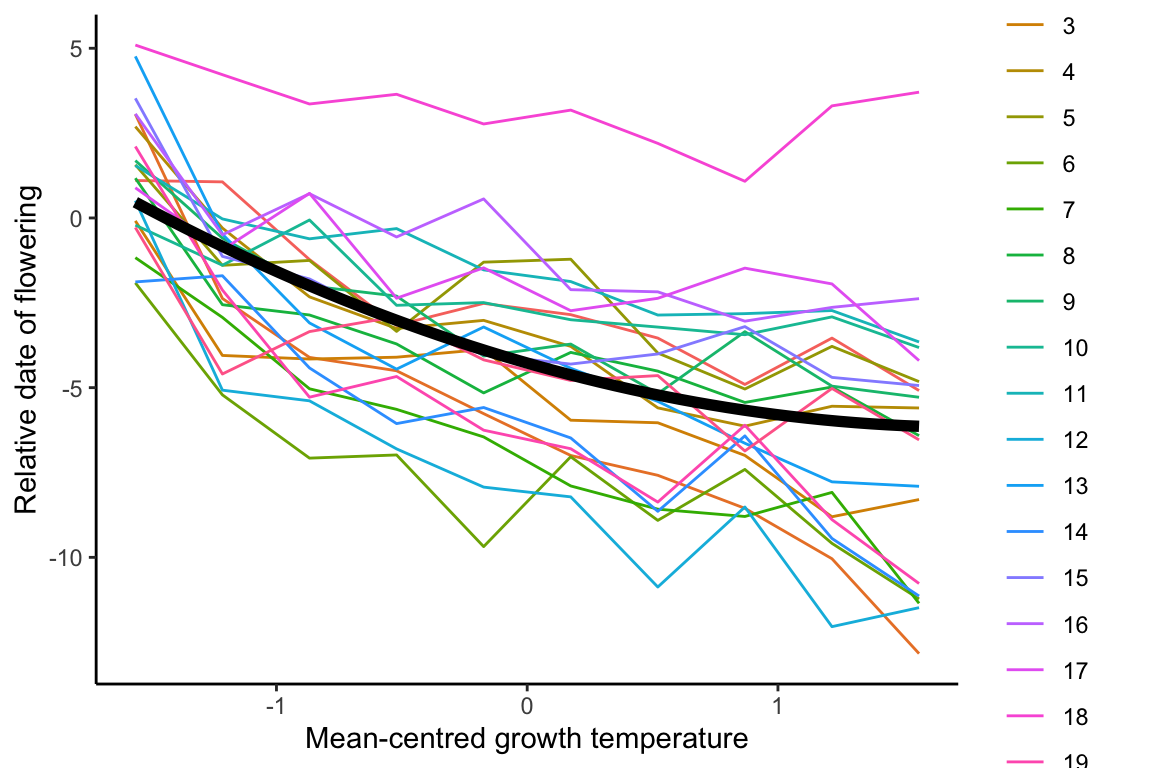
## 'log Lik.' 0.0123132 (df=5)## df AIC
## model1.1 4 998.2138
## model1.2 5 993.9486This model’s R^2 value is 0.37, which is marginal improvement in model fit over the linear model.
The p-value is 0.012, marginal significant.
To further improve the model, the overall population-level reaction norm could be added with an additional term of (1|genotype), which allows different genotypes to have different intercepts on the y-axis.
building quadratic fixed effects with random intercepts model
## Linear mixed model fit by maximum likelihood  ['lmerMod']
## Formula: relativedate ~ poly(ctemperature, 2, raw = T) + (1 | loc) + (1 |
##     genotype)
##    Data: flowerdata
##
##      AIC      BIC   logLik deviance df.resid
##    757.9    777.7   -373.0    745.9      194
##
## Scaled residuals:
##     Min      1Q  Median      3Q     Max
## -3.2264 -0.5963  0.0544  0.5306  3.3112
##
## Random effects:
##  Groups   Name        Variance Std.Dev.
##  genotype (Intercept) 6.2666   2.5033
##  loc      (Intercept) 0.1943   0.4408
##  Residual             1.5941   1.2626
## Number of obs: 200, groups:  genotype, 20; loc, 10
##
## Fixed effects:
##                                 Estimate Std. Error t value
## (Intercept)                      -4.2757     0.6132  -6.973
## poly(ctemperature, 2, raw = T)1  -2.1124     0.1659 -12.730
## poly(ctemperature, 2, raw = T)2   0.5890     0.1889   3.119
##
## Correlation of Fixed Effects:
##             (Intr) p(,2,r=T)1
## pl(,2,r=T)1  0.000
## pl(,2,r=T)2 -0.306  0.000
## R2m R2c
## [1,] 0.3699661 0.8753124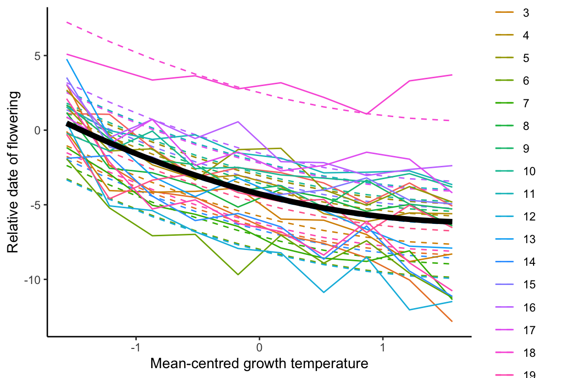
## 'log Lik.' 0 (df=6)## df AIC
## model1.1 4 998.2138
## model1.2 5 993.9486
## model1.3 6 757.9457buliding quadratic fixed effects with linear random regression model
## Linear mixed model fit by maximum likelihood  ['lmerMod']
## Formula: relativedate ~ poly(ctemperature, 2, raw = T) + (1 | loc) + (1 +
##     ctemperature | genotype)
##    Data: flowerdata
##
##      AIC      BIC   logLik deviance df.resid
##    685.2    711.5   -334.6    669.2      192
##
## Scaled residuals:
##      Min       1Q   Median       3Q      Max
## -2.39983 -0.57568 -0.02542  0.44597  2.64265
##
## Random effects:
##  Groups   Name         Variance Std.Dev. Corr
##  genotype (Intercept)  6.3413   2.5182
##           ctemperature 0.6190   0.7868   0.80
##  loc      (Intercept)  0.2383   0.4882
##  Residual              0.8806   0.9384
## Number of obs: 200, groups:  genotype, 20; loc, 10
##
## Fixed effects:
##                                 Estimate Std. Error t value
## (Intercept)                      -4.2757     0.6178  -6.921
## poly(ctemperature, 2, raw = T)1  -2.1124     0.2436  -8.672
## poly(ctemperature, 2, raw = T)2   0.5890     0.1917   3.072
##
## Correlation of Fixed Effects:
##             (Intr) p(,2,r=T)1
## pl(,2,r=T)1  0.529
## pl(,2,r=T)2 -0.309  0.000
## R2m R2c
## [1,] 0.3693535 0.9312344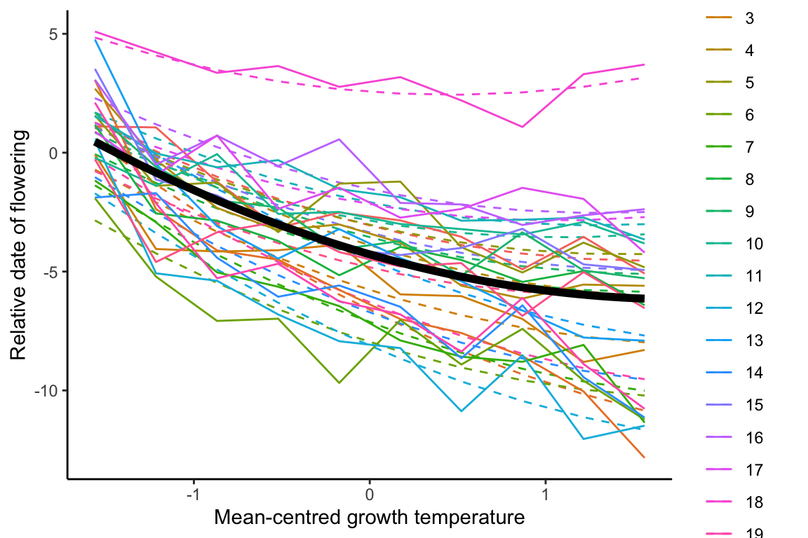
## 'log Lik.' -372.9728 (df=6)## 'log Lik.' -334.5753 (df=8)## 'log Lik.' 0 (df=8)## df AIC
## model1.1 4 998.2138
## model1.2 5 993.9486
## model1.3 6 757.9457
## model1.4 8 685.1506Using BLUPs to rank plasticity
Fitting data to the model also allows us to rank genotyeps in terms of their plasticity.
We can extract BLUPs to rank which genotypes are least or most plastic.
BLUPs can be extracted from a mixed-effects models by calling ranef().
Here, BLUPs represent the response of a given genotype to the fixed effect of temperature as the difference between that genotype’s predicted response and the population-level average predicted response.
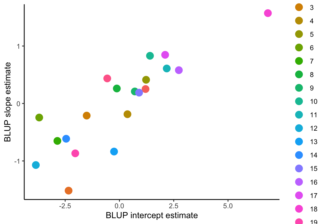
In the case of a random regression model (as in model1.4), there are two random effects: the intercept and the slope.
The BLUP intercept term indicates the difference in genotype elevation relative to the population-average, so more positive values of BLUP intercept indicate that the genotype’s reaction norm occurs above the population-level average and negative values are below the population-level average.
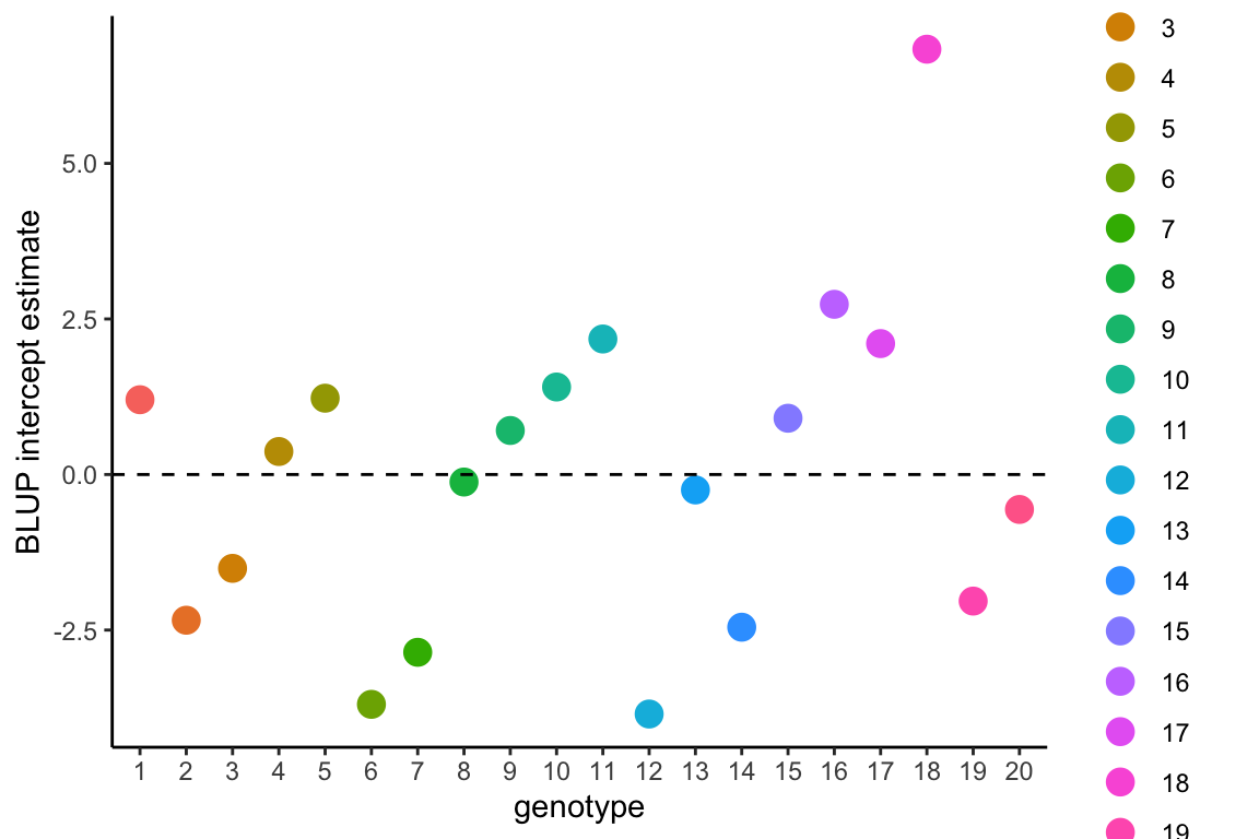
The BLUP intercept values are not a measure of plasticity, but these values may be correlated with BLUP slope values and otherwise may be a parameter of interest for comparing among genotypes.
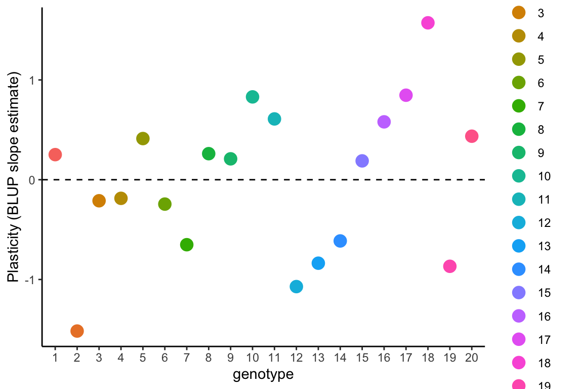
The BLUP slope estimate is the difference in slope (relative steepness of change) between the population-level average response and the response of the individual genotype.
Here, that is the difference in slope of the relative date of flowering for each value of temperature relative to the population-level average slope。
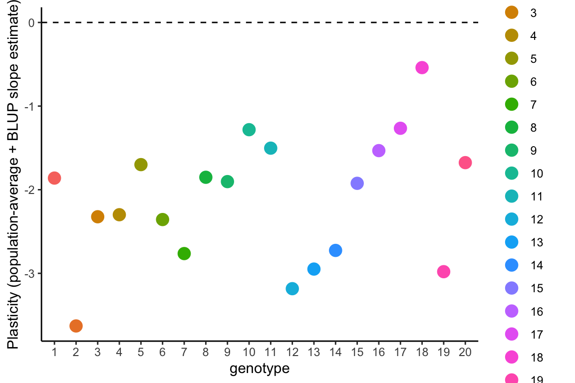
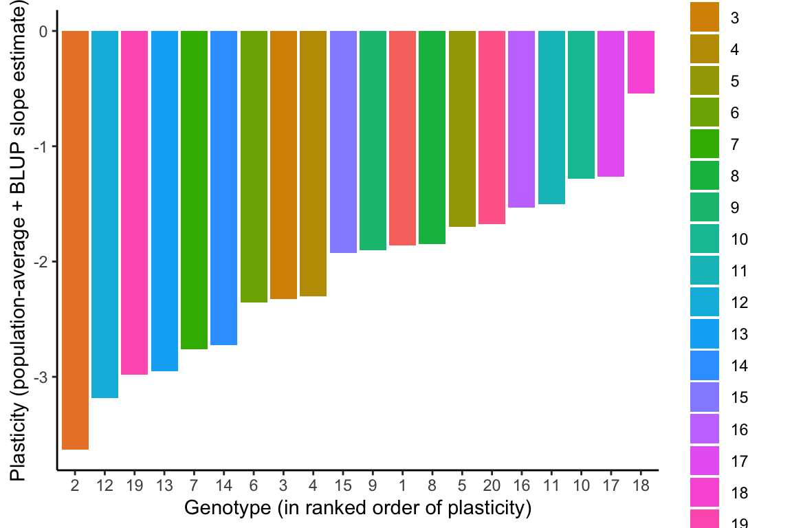
Because the population-level average response is negative overall, all genotypes have a negative slope when the BLUP slope estimates are added to the population-level average slope estimate from model1.4 (
The BLUP intercept and slope estimates are sometimes correlated. The correlation coefficient is given in the random effects correlation from the model1.4 summary, which is 0.8. This positive relationship can clearly be seen in the figure below, where the genotype with the most positive BLUP slope estimate has the highest positive intercept.
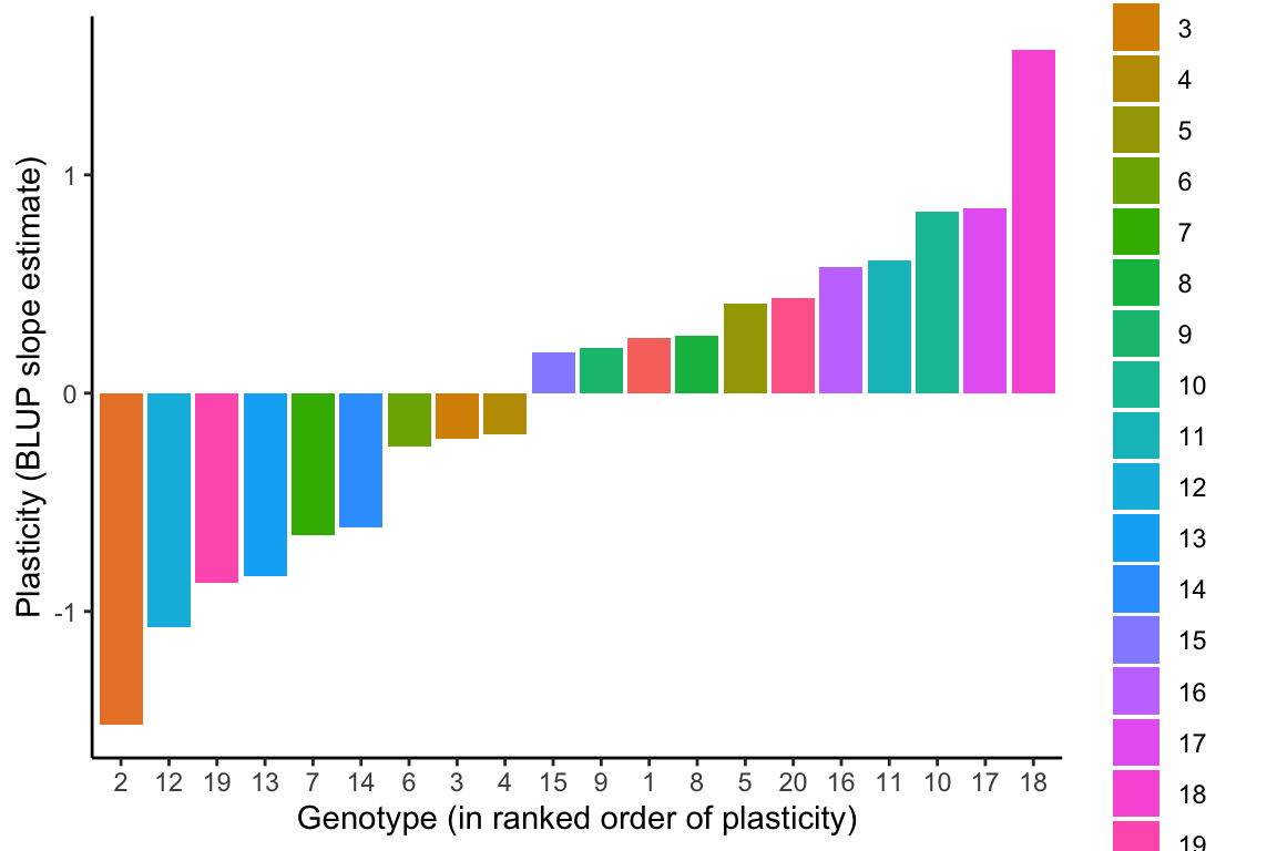
The genotypes can then be ranked in order of plasticity by BLUP slope estimates. Because the population-level average response is negative, the most negative BLUP slope estimates represent steeper reaction norm slopes and hence greater plasticity, and more positive BLUP slope estimates represent flatter reaction norms and less plasticity in the relative date of flowering in response to growth temperatures.
References
- Arnold, Pieter A., Loeske EB Kruuk, and Adrienne B. Nicotra. “How to analyse plant phenotypic plasticity in response to a changing climate.” New Phytologist 222.3 (2019): 1235-1241.
## R version 4.1.3 (2022-03-10)
## Platform: x86_64-apple-darwin17.0 (64-bit)
## Running under: macOS Big Sur/Monterey 10.16
##
## Matrix products: default
## BLAS:   /Library/Frameworks/R.framework/Versions/4.1/Resources/lib/libRblas.0.dylib
## LAPACK: /Library/Frameworks/R.framework/Versions/4.1/Resources/lib/libRlapack.dylib
##
## locale:
## [1] en_US.UTF-8/en_US.UTF-8/en_US.UTF-8/C/en_US.UTF-8/en_US.UTF-8
##
## attached base packages:
## [1] stats     graphics  grDevices utils     datasets  methods   base
##
## other attached packages:
##  [1] lme4_1.1-28     Matrix_1.4-0    MuMIn_1.46.0    forcats_0.5.1
##  [5] stringr_1.4.0   dplyr_1.0.8     purrr_0.3.4     readr_2.1.2
##  [9] tidyr_1.2.0     tibble_3.1.6    ggplot2_3.4.0   tidyverse_1.3.1
## [13] knitr_1.37
##
## loaded via a namespace (and not attached):
##  [1] Rcpp_1.0.8       lubridate_1.8.0  lattice_0.20-45  assertthat_0.2.1
##  [5] digest_0.6.29    utf8_1.2.2       R6_2.5.1         cellranger_1.1.0
##  [9] backports_1.4.1  reprex_2.0.1     stats4_4.1.3     evaluate_0.15
## [13] highr_0.9        httr_1.4.2       blogdown_1.17.2  pillar_1.7.0
## [17] rlang_1.0.6      readxl_1.4.0     minqa_1.2.4      rstudioapi_0.13
## [21] nloptr_2.0.0     jquerylib_0.1.4  rmarkdown_2.13   labeling_0.4.2
## [25] splines_4.1.3    munsell_0.5.0    broom_0.7.12     compiler_4.1.3
## [29] modelr_0.1.8     xfun_0.39        pkgconfig_2.0.3  htmltools_0.5.2
## [33] tidyselect_1.1.1 bookdown_0.25    fansi_1.0.2      crayon_1.5.0
## [37] tzdb_0.2.0       dbplyr_2.1.1     withr_2.5.0      MASS_7.3-55
## [41] grid_4.1.3       nlme_3.1-155     jsonlite_1.8.0   gtable_0.3.0
## [45] lifecycle_1.0.3  DBI_1.1.2        magrittr_2.0.2   scales_1.2.1
## [49] cli_3.5.0        stringi_1.7.8    farver_2.1.0     fs_1.5.2
## [53] xml2_1.3.3       bslib_0.3.1      ellipsis_0.3.2   generics_0.1.2
## [57] vctrs_0.5.1      boot_1.3-28      tools_4.1.3      glue_1.6.1
## [61] hms_1.1.1        fastmap_1.1.0    yaml_2.3.4       colorspace_2.0-2
## [65] rvest_1.0.2      haven_2.4.3      sass_0.4.0