When I was doing regression analysis, people suggested that I should try ‘linear mixed model’ to better account for the non-independence observations in my dataset or to better control for confounding variables.
I was reading some papers related to linear mixed model, paper1 paper2, I felt very inspired, but when it came to practical research, the real thing I need is a tool that can ‘make things happen’, or can help me build the linear mixed model, estimate parameter, partition the variance and get the significance value.
The more I read, the more I feel there is no ‘simple’ or ‘final’ answer to these questions, like I didn’t know the degree of freedom of a model could be a decimal instead of a integer, and it is a ‘huge’ thing how to properly estimate the number of freedom in a mixed model, which will affect the following model testing. paper3 paper4
After some exploration, I decided I would stop struggling and barely keeping breathing in the water, I’ll see if there is any already-built and easy-to-wear life-vest, put it on, float in the water, as long as it doesn’t get poked.
So, one thing I frequently get asked when presenting data in lab meeting is how much variance each variable in the linear mixed model could explain, no matter it’s a fixed effect or random effect.
After some trying, I find this variancePartition R package really helpful, it is built upon ‘lme4’ package and nicely wrap up ‘lmer’ function output (from lme4 package) into simple, intuitive results.
It has a very nice documentation and is easy to get started.
Hands-on Time~~
if (!require("variancePartition")){BiocManager::install("variancePartition")}

library(variancePartition)
library(lme4)

# load the data we are gonna play with
data(varPartData)
glimpse(geneExpr) #200gene X 100samples matrix
## num [1:200, 1:100] -7.67 0.579 1.748 -2.813 8.535 ...
## - attr(*, "dimnames")=List of 2
## ..$ : chr [1:200] "gene1" "gene2" "gene3" "gene4" ...
## ..$ : chr [1:100] "s1" "s2" "s3" "s4" ...glimpse(info) #sample meta information## Rows: 100
## Columns: 6
## $ ID <fct> s1, s2, s3, s4, s5, s6, s7, s8, s9, s10, s11, s12, s13, s14…
## $ Individual <fct> 1, 5, 9, 13, 18, 22, 26, 30, 34, 38, 42, 46, 50, 55, 59, 63…
## $ Tissue <fct> A, C, C, A, A, B, A, A, B, B, C, A, A, B, B, C, C, A, A, C,…
## $ Batch <fct> 1, 4, 2, 3, 1, 4, 1, 4, 1, 2, 2, 2, 4, 4, 2, 2, 4, 2, 2, 2,…
## $ Age <int> 44, 42, 49, 48, 56, 43, 37, 48, 50, 56, 39, 60, 54, 57, 50,…
## $ Height <dbl> 157.4983, 196.6674, 189.4191, 156.2051, 178.4908, 175.4234,…# fit regression model for the first gene
fit <- lmer(geneExpr[1,] ~ Age + (1|Individual) + (1|Tissue), data=info, REML=FALSE )
# use fixef() and ranef() to get estimated.coeff
fixef(fit)## (Intercept) Age
## -10.600245932 0.003119818ranef(fit)## $Individual
## (Intercept)
## 1 1.2231161
## 5 -7.7886575
## 9 1.0439504
## 13 2.0211472
## 18 1.3756169
## 22 -1.9321541
## 26 0.7661554
## 30 -8.0038302
## 34 0.3708665
## 38 -0.1993725
## 42 4.8459164
## 46 3.2687786
## 50 1.6290156
## 55 0.4767442
## 59 0.4385986
## 63 3.4730313
## 67 -4.6375776
## 71 2.5240272
## 75 -0.2526089
## 79 -3.8195473
## 84 2.0980820
## 88 -1.1621572
## 92 4.8074212
## 96 -1.0930034
## 100 -1.4735590
##
## $Tissue
## (Intercept)
## A 0.48656898
## B -0.57527535
## C 0.08870637
##
## with conditional variances for "Individual" "Tissue"calcVarPart(fit)## Individual Tissue Age Residuals
## 8.903140e-01 2.468013e-02 4.354738e-05 8.496235e-02sum(calcVarPart(fit)) #the total.var normalized to 100 ## [1] 1# manually check above 'fit'
fit## Linear mixed model fit by maximum likelihood ['lmerMod']
## Formula: geneExpr[1, ] ~ Age + (1 | Individual) + (1 | Tissue)
## Data: info
## AIC BIC logLik deviance df.resid
## 395.1549 408.1807 -192.5774 385.1549 95
## Random effects:
## Groups Name Std.Dev.
## Individual (Intercept) 3.2881
## Tissue (Intercept) 0.5475
## Residual 1.0158
## Number of obs: 100, groups: Individual, 25; Tissue, 3
## Fixed Effects:
## (Intercept) Age
## -10.60025 0.00312fit.summary<-summary(fit)
# begin manually 'deconstructing' all variance components
# extract the variance of the random effect which is not captured by the fixed effects.
(var.random <- as.numeric(fit.summary$varcor))## [1] 10.8118122 0.2997111names(var.random)<-names(fit.summary$varcor)
# extract the residual variance
(var.residual <- attr(VarCorr(fit), "sc")^2) ## [1] 1.031768names(var.residual)<-'Residuals';
# use the variance of predicted values in a linear model involving the fixed effect alone to 'approximate' variance component that explained by fixed effects.
X<-model.matrix(~-1+Age,data=info)
var.fixed<-var(X %*% fixef(fit)[[2]])[[1]]
names(var.fixed)='Age'
# total variance in the response variable(gene1 expression values across all samples)
var(geneExpr[1,])## [1] 12.55749sum(var.random+var.fixed+var.residual) ## [1] 13.17613c(var.random,var.fixed,var.residual)/sum(var.random+var.residual+var.fixed)## Individual Tissue Age Residuals
## 8.205607e-01 2.274652e-02 4.054099e-05 7.830583e-02calcVarPart(fit) #not exactly... but pretty close## Individual Tissue Age Residuals
## 8.903140e-01 2.468013e-02 4.354738e-05 8.496235e-02# refit the first gene expression with two fixed effects
fit <- lmer(geneExpr[1,] ~ Age + Height+(1|Individual) + (1|Tissue), info, REML=FALSE )
calcVarPart(fit)## Individual Tissue Age Height Residuals
## 8.900647e-01 2.512262e-02 5.359814e-05 1.372418e-04 8.462180e-02# manually check above 'fit'
fit.summary<-summary(fit)
(var.random <- as.numeric(fit.summary$varcor))## [1] 10.8240167 0.3055145names(var.random)<-names(fit.summary$varcor)
(var.residual <- attr(VarCorr(fit), "sc")^2) ## [1] 1.02908names(var.residual)<-'Residuals';
X<-model.matrix(~-1+Age+Height,data=info)
var.fixed1<-var(X[,1,drop=F] * fixef(fit)[[2]])[[1]]
var.fixed2<-var(X[,1,drop=F] * fixef(fit)[[3]])[[1]]
names(var.fixed1)='Age'
names(var.fixed2)='Height'
var(geneExpr[1,])## [1] 12.55749sum(var.random+var.fixed1+var.fixed2+var.residual) ## [1] 13.1899c(var.random,var.fixed1,var.fixed2,var.residual)/sum(var.random+var.fixed1+var.fixed2+var.residual) ## Individual Tissue Age Height Residuals
## 8.206291e-01 2.316276e-02 4.947978e-05 3.430493e-05 7.802029e-02calcVarPart(fit) #yeah... there is certainly some difference for fixed effect## Individual Tissue Age Height Residuals
## 8.900647e-01 2.512262e-02 5.359814e-05 1.372418e-04 8.462180e-02# refit again...
fit <- lmer(geneExpr[1,] ~ Age + Height+(1|Batch)+(1|Individual) + (1|Tissue), info, REML=FALSE )
calcVarPart(fit)## Batch Individual Tissue Age Height Residuals
## 1.581599e-04 8.901228e-01 2.513129e-02 5.550236e-05 1.369134e-04 8.439533e-02# manually check above 'fit'
fit.summary<-summary(fit)
(var.random <- as.numeric(fit.summary$varcor))## [1] 10.834860167 0.001925173 0.305906112names(var.random)<-names(fit.summary$varcor)
(var.residual <- attr(VarCorr(fit), "sc")^2) ## [1] 1.027287names(var.residual)<-'Residuals';
X<-model.matrix(~-1+Age+Height,data=info)
var.fixed1<-var(X[,1,drop=F] * fixef(fit)[[2]])[[1]]
var.fixed2<-var(X[,1,drop=F] * fixef(fit)[[3]])[[1]]
names(var.fixed1)='Age'
names(var.fixed2)='Height'
var(geneExpr[1,])## [1] 12.55749sum(var.random+var.fixed1+var.fixed2+var.residual) ## [1] 14.22794c(var.random,var.fixed1,var.fixed2,var.residual)/sum(var.random+var.fixed1+var.fixed2+var.residual) ## Individual Batch Tissue Age Height Residuals
## 7.615201e-01 1.353094e-04 2.150038e-02 4.754064e-05 3.175350e-05 7.220210e-02calcVarPart(fit)#crap... the difference becomes bigger...## Batch Individual Tissue Age Height Residuals
## 1.581599e-04 8.901228e-01 2.513129e-02 5.550236e-05 1.369134e-04 8.439533e-02I was just curious how they ‘actually’ partition the variance and began to look at their source code. Btw, I think learning through the source code is an effective way and I share something from the book Advanced R by one of my favorite statisticians Hadley Wickham as below:
1.5 Meta-techniques
There are two meta-techniques that are tremendously helpful for improving your skills as an R programmer: reading source code and adopting a scientific mindset.
- Reading source code is important because it will help you write better code. A great place to start developing this skill is to look at the source code of the functions and packages you use most often. You’ll find things that are worth emulating in your own code and you’ll develop a sense of taste for what makes good R code. You will also see things that you don’t like, either because its virtues are not obvious or it offends your sensibilities. Such code is nonetheless valuable, because it helps make concrete your opinions on good and bad code.
- A scientific mindset is extremely helpful when learning R. If you don’t understand how something works, you should develop a hypothesis, design some experiments, run them, and record the results. This exercise is extremely useful since if you can’t figure something out and need to get help, you can easily show others what you tried. Also, when you learn the right answer, you’ll be mentally prepared to update your world view.
So back to topic, I checked their source code to make sure they were not playing tricks!
From my understanding,
the basic assumption here is: total.var = random.var + fixed.var + error/residue.
The procedures of getting values for above terms are:
random.var: variance explained by random predictors, are extracted from the output of lmer() functionerror/residue: variance failed to be captured by this mixed model, are extracted from the output of lmer() functionfixed var: This is the trickly part!!! how to get variance explained by fixed predictors.
One way to get some numbers out is:
Since mixed model estimate beta coefficients for fixed predictors, they calculate fitted response values with each fixed predictor alone.
Say you have two predictors, with each predictor alone, you get a set of fitted values.
- then with the fitted values using predictor 1 alone, you calculate the variance.
- with the fitted values using predictor 2 alone, you calculate the variance.
These two variance values represent the variance explained by fixed predictors.
I did some validation shown as above and compared my calculation with the function’s output: summed up each component explained variance and calculated the response variable variance, check if they satisfy total.var = random.var + fixed.var + error/residue, as well as the explained variance propotion.
It seems with only one fixed effect, the discrepancy is not that large, but when I involve more fixed effects in the mixed model, my way of calculating the variance components begin to drift away from their results…
I think it’s OK and it may be due to my crappy ‘validation’ approach,( also shown here). In the package souce code, their implementation is more complicated and delicate.
Finally, some more code demonstrating the variancePartition package utility (just copy and paste from the package documentation)
# model form
form <- ~ Age + (1|Individual) + (1|Tissue) + (1|Batch)
# model fitting and variance extraction in one step
varPart <- fitExtractVarPartModel( geneExpr, form, info )

# sort result
vp <- sortCols( varPart )
# and plot
plotPercentBars( vp[1:10,] )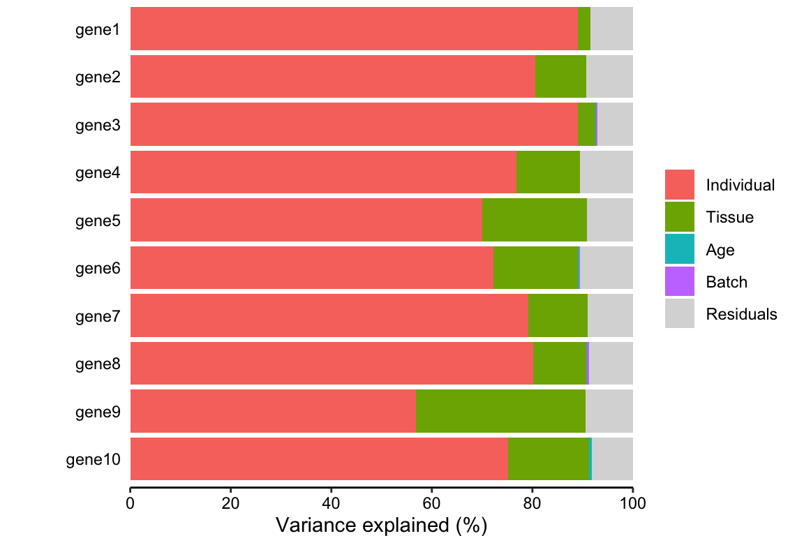
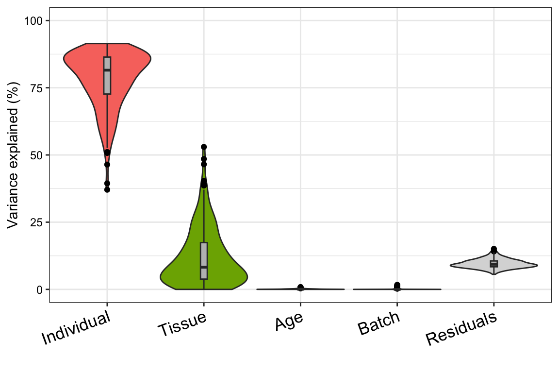
# violin plot of each variable contribution to total variance
plotVarPart( vp )