All datasets are downloaded here: http://www.hiercourse.com/mixedeffects.html
The code is extracted from this tutorial: http://www.hiercourse.com/docs/Rnotes_mixed.pdf
dataset1: individual-level variation in tree canopy gradients
data inspection
pref<-read.csv("prefdata.csv")
head(pref)
## ID species dfromtop totheight height LMA narea
## 1 FP11 Pinus ponderosa 8.88 22.40 13.52 319.4472 2.779190
## 2 FP11 Pinus ponderosa 0.62 22.40 21.78 342.7948 4.010700
## 3 FP11 Pinus ponderosa 4.72 22.40 17.68 329.5399 3.365579
## 4 FP15 Pinus ponderosa 2.74 27.69 24.95 312.4467 3.682907
## 5 FP15 Pinus ponderosa 5.48 27.69 22.21 278.4037 2.524224
## 6 FP15 Pinus ponderosa 8.40 27.69 19.29 255.9716 2.351546pref$species=factor(pref$species)
levels(pref$species)## [1] "Pinus monticola" "Pinus ponderosa"# two tree species
# interested in using species and dfromtop to predict LMA
ggplot(pref,aes(x=dfromtop,y=LMA,col=species))+
geom_point()+theme_bw()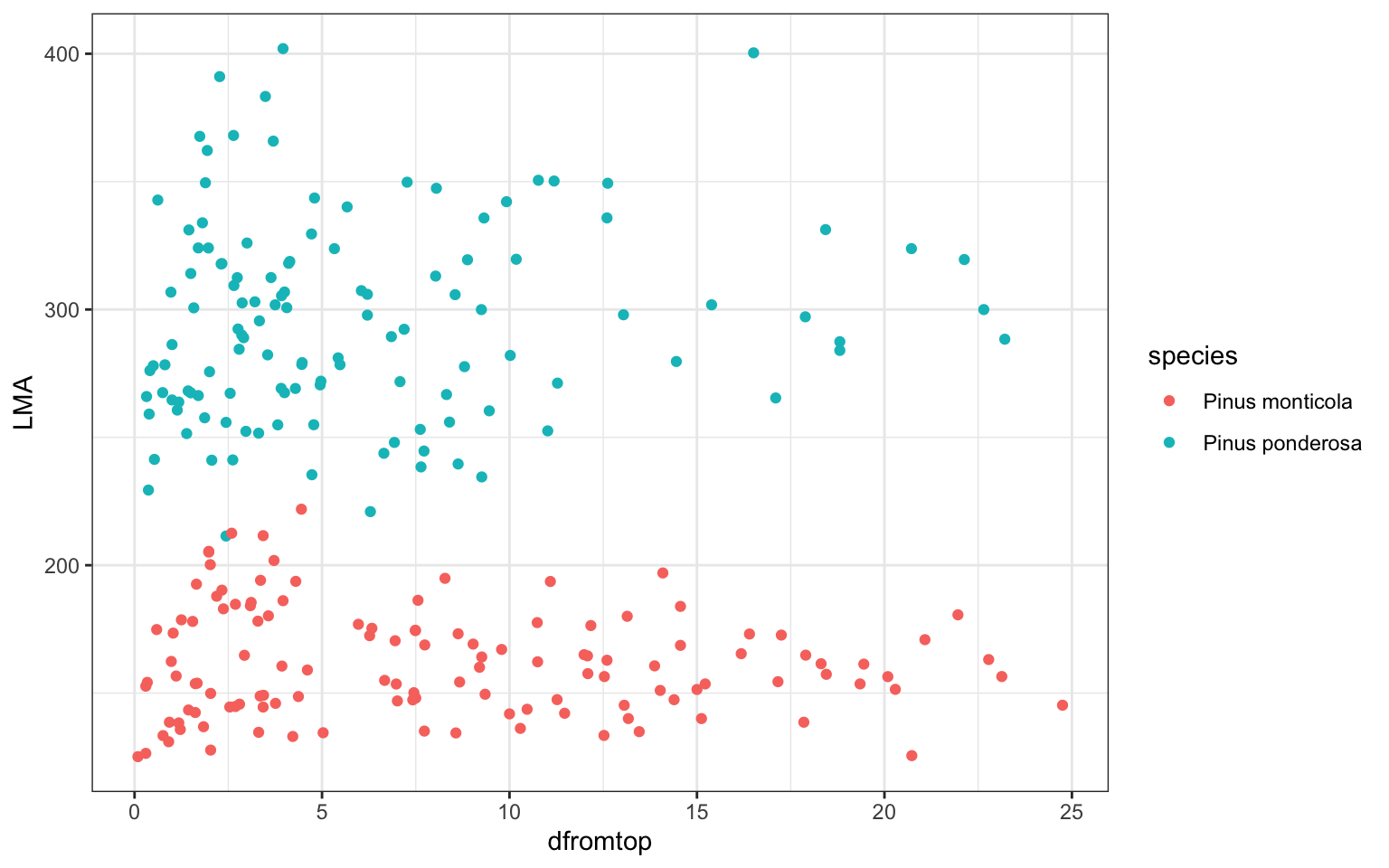
# but here, not each point is a independent tree
# as each tree have more than one mearsurements
ggplot(pref,aes(x=dfromtop,y=LMA,col=species))+
  geom_point()+theme_bw()+facet_wrap(.~ID)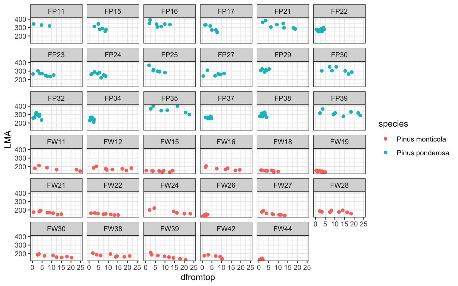
ggplot(pref,aes(x=dfromtop,y=LMA,col=species))+
  geom_point()+theme_bw()+geom_line(aes(group=ID))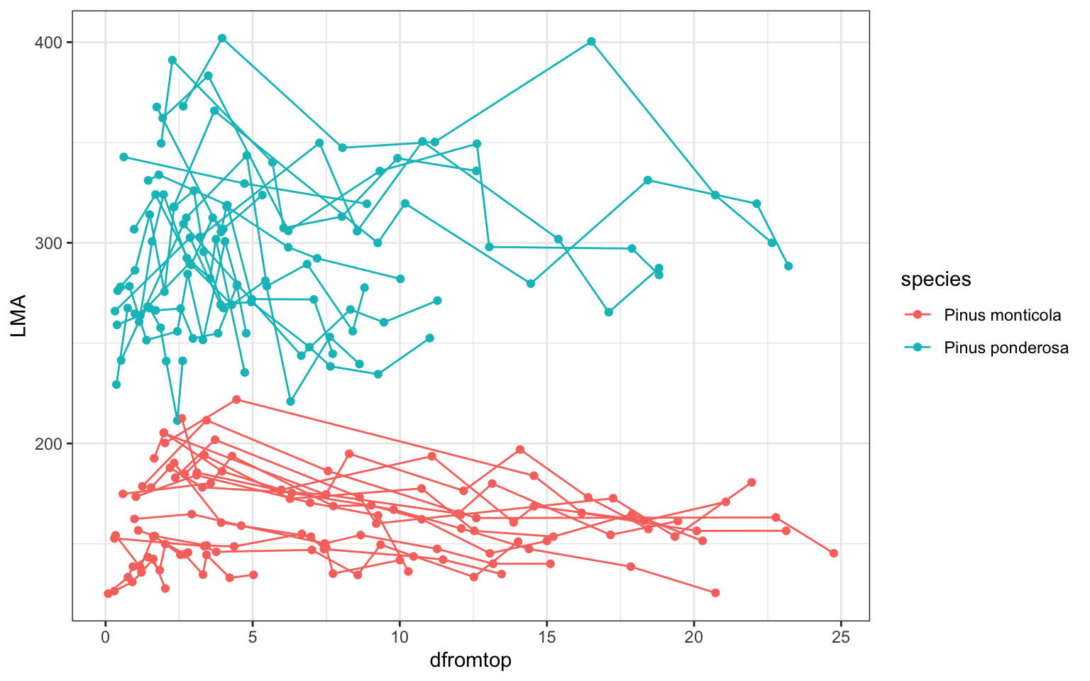
### dataset description: two species, each has some tree individuals
# and there are repeated measures for each individual
# can we use one 'common model framework' to describe all of them
to start with, fit a linear regression by species (ignoring individual-level variation)
lm1 <- lm(LMA ~ species + dfromtop + species:dfromtop, data=pref)
# Plot predictions
library(visreg)
visreg(lm1, "dfromtop", by="species", overlay=TRUE)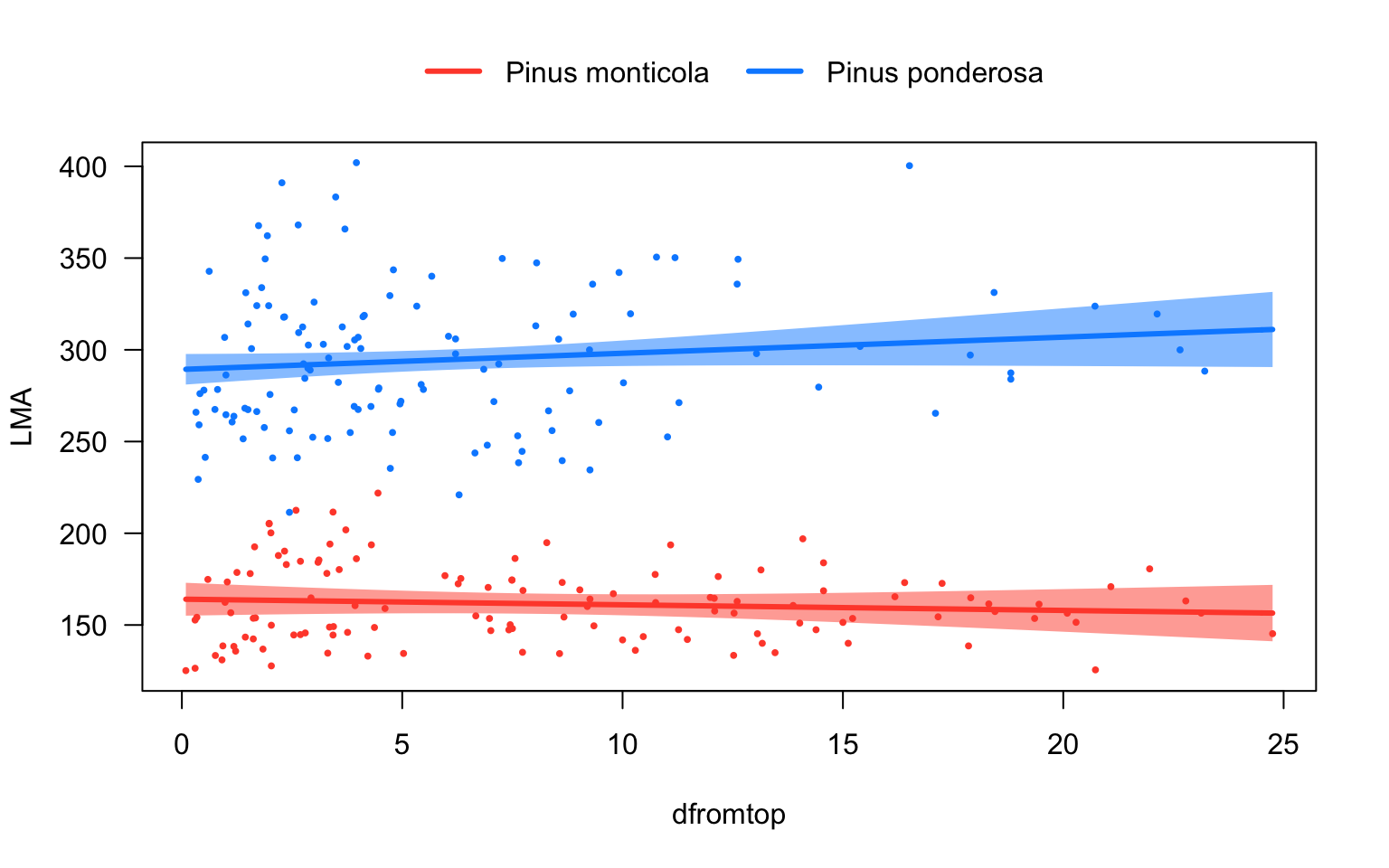
tricky thing about ‘anova’, use ‘Anova’ instead!
anova(lm1)## Analysis of Variance Table
##
## Response: LMA
## Df Sum Sq Mean Sq F value Pr(>F)
## species 1 1101739 1101739 1121.5735 <2e-16 ***
## dfromtop 1 258 258 0.2623 0.6090
## species:dfromtop 1 2880 2880 2.9322 0.0881 .
## Residuals 245 240667 982
## ---
## Signif. codes: 0 '***' 0.001 '**' 0.01 '*' 0.05 '.' 0.1 ' ' 1lm1.1 <- lm(LMA ~ dfromtop+species+species:dfromtop, data=pref)
anova(lm1.1)## Analysis of Variance Table
##
## Response: LMA
## Df Sum Sq Mean Sq F value Pr(>F)
## dfromtop 1 32406 32406 32.9897 2.734e-08 ***
## species 1 1069590 1069590 1088.8462 < 2.2e-16 ***
## dfromtop:species 1 2880 2880 2.9322 0.0881 .
## Residuals 245 240667 982
## ---
## Signif. codes: 0 '***' 0.001 '**' 0.01 '*' 0.05 '.' 0.1 ' ' 1Note that the order of the variables entered in the model matters because each next term is tested against a model that includes all terms preceding it (so-called Type-I tests). These standard tests with anova are sequential tests, which is perhaps not the most intuitive behaviour. #In many cases it is more intuitive to use so-called Type-II tests, in which each main effect is tested against a model that includes all other terms. We can use Anova (from the car package) to do this.
to circumvent this, use ‘Anova’ from ‘car’ package
library(car)
Anova(lm1)
## Anova Table (Type II tests)
##
## Response: LMA
## Sum Sq Df F value Pr(>F)
## species 1069590 1 1088.8462 <2e-16 ***
## dfromtop 258 1 0.2623 0.6090
## species:dfromtop 2880 1 2.9322 0.0881 .
## Residuals 240667 245
## ---
## Signif. codes: 0 '***' 0.001 '**' 0.01 '*' 0.05 '.' 0.1 ' ' 1Anova(lm1.1)## Anova Table (Type II tests)
##
## Response: LMA
## Sum Sq Df F value Pr(>F)
## dfromtop 258 1 0.2623 0.6090
## species 1069590 1 1088.8462 <2e-16 ***
## dfromtop:species 2880 1 2.9322 0.0881 .
## Residuals 240667 245
## ---
## Signif. codes: 0 '***' 0.001 '**' 0.01 '*' 0.05 '.' 0.1 ' ' 1do lm many times: fit each LMA~dfromtop for each tree separately
# fit linear regression by tree ('ID')
library(lme4)
lmlis1 <- lmList(LMA ~ dfromtop | ID, data=pref)
# Extract coefficients (intercepts and slopes) for each tree
liscoef <- coef(lmlis1)
# load plottix for the 'ablineclip' function, which clips lines within the range of x
library(plotrix)
# split pref by tree (prefsp is a list)
prefsp <- split(pref, pref$ID)
names(prefsp)
## [1] "FP11" "FP15" "FP16" "FP17" "FP21" "FP22" "FP23" "FP24" "FP25" "FP27"
## [11] "FP29" "FP30" "FP32" "FP34" "FP35" "FP37" "FP38" "FP39" "FW11" "FW12"
## [21] "FW15" "FW16" "FW18" "FW19" "FW21" "FW22" "FW24" "FW26" "FW27" "FW28"
## [31] "FW30" "FW38" "FW39" "FW42" "FW44"rownames(liscoef)## [1] "FP11" "FP15" "FP16" "FP17" "FP21" "FP22" "FP23" "FP24" "FP25" "FP27"
## [11] "FP29" "FP30" "FP32" "FP34" "FP35" "FP37" "FP38" "FP39" "FW11" "FW12"
## [21] "FW15" "FW16" "FW18" "FW19" "FW21" "FW22" "FW24" "FW26" "FW27" "FW28"
## [31] "FW30" "FW38" "FW39" "FW42" "FW44"sum(rownames(liscoef)==names(prefsp))## [1] 35# Plot
palette(c("red","blue"))
with(pref, plot(dfromtop, LMA, col=species, pch=16, cex=0.8))
for(i in 1:length(prefsp)){
# Find min and max values of dfromtop, to send to ablineclip
xmin <- min(prefsp[[i]]$dfromtop)
xmax <- max(prefsp[[i]]$dfromtop)
# add regression lines
ablineclip(liscoef[i,1], liscoef[i,2], x1=xmin, x2=xmax,
col=prefsp[[i]]$species)
}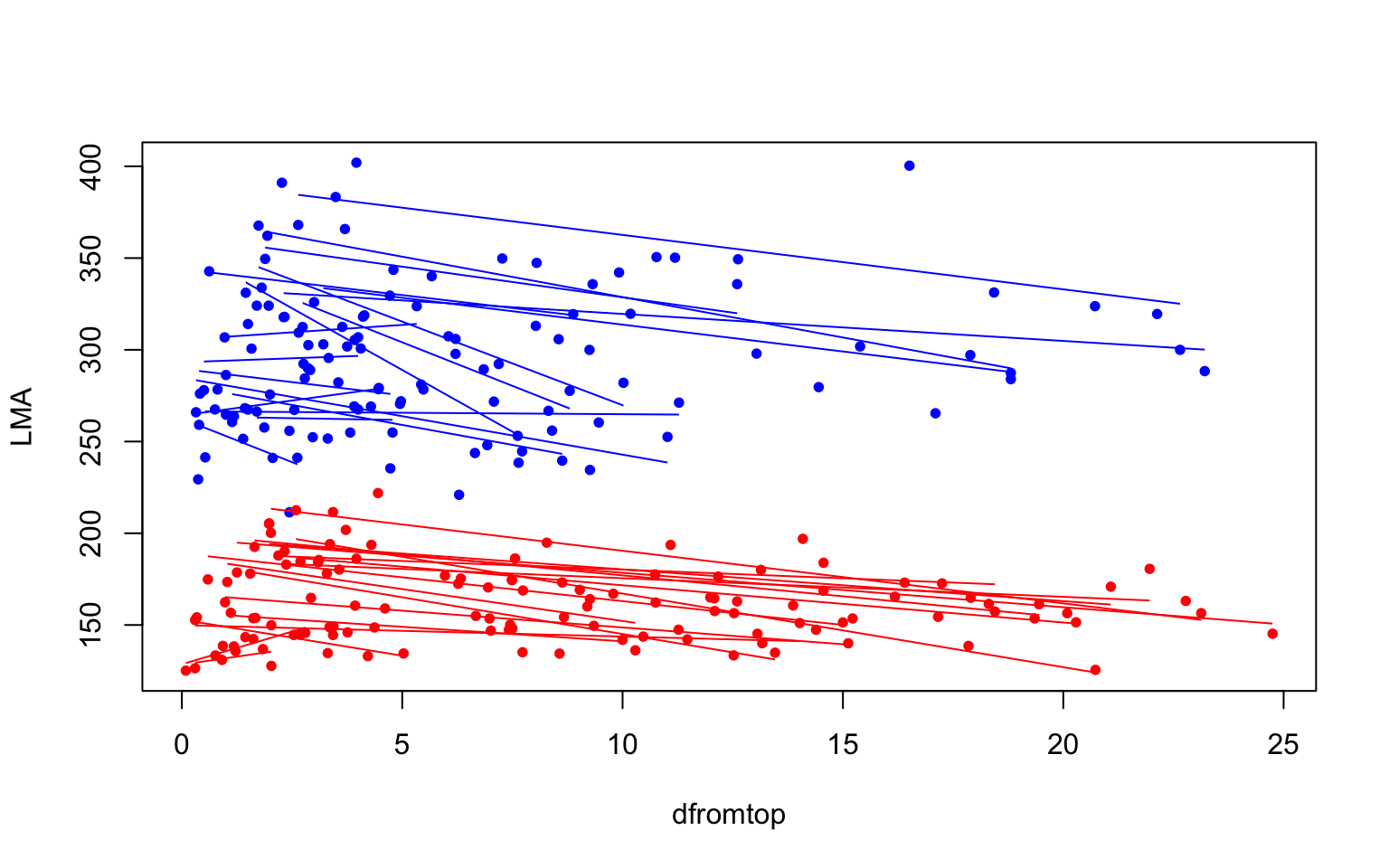
Messages from the above plots:
- Intercepts vary a lot between trees
- There seems to be a negative relationship for many trees
- It seems there is less variation between slopes than intercepts
fit mixed models and compare them
fit two models: one with a random intercept only, and one with a random intercept and slope.
When we fit a mixed-effects model, not only do we get an estimate of the variance (or standard de- viation) of the random effects, we also get estimates of this random effect for each individual. These estimates are known as the BLUPs (best linear unbiased predictors).
# explore random structure in data
library(lme4)
# Random intercept only
pref_m1 <- lmer(LMA ~ species + dfromtop + species:dfromtop + (1|ID), data=pref)
# Random intercept and slope
pref_m2 <- lmer(LMA ~ species + dfromtop + species:dfromtop + (dfromtop|ID), data=pref)
# there is warning message, but the model still gets built

VarCorr(pref_m1)
## Groups Name Std.Dev.
## ID (Intercept) 30.714
## Residual 18.088VarCorr(pref_m2)## Groups Name Std.Dev. Corr
## ID (Intercept) 31.36660
## dfromtop 0.47658 -0.305
## Residual 17.96297fixef(pref_m1)## (Intercept) speciesPinus ponderosa
## 177.9436940 134.9771944
## dfromtop speciesPinus ponderosa:dfromtop
## -2.0001352 -0.8197089head(ranef(pref_m1)[[1]])## (Intercept)
## FP11 27.822753
## FP15 -2.449878
## FP16 43.500992
## FP17 -4.529720
## FP21 41.593278
## FP22 -32.351729fixef(pref_m2)## (Intercept) speciesPinus ponderosa
## 177.9024666 135.0267826
## dfromtop speciesPinus ponderosa:dfromtop
## -1.9609636 -0.8277069head(ranef(pref_m2)[[1]])## (Intercept) dfromtop
## FP11 28.203671 -0.1005236
## FP15 -1.876980 -0.1086252
## FP16 44.415213 -0.1653518
## FP17 -3.478808 -0.2183607
## FP21 44.908819 -0.3422695
## FP22 -33.001675 0.1942158### compare mixed model (anova.merMod)
AIC(pref_m1,pref_m2) #AIC## df AIC
## pref_m1 6 2251.997
## pref_m2 8 2255.735anova(pref_m1, pref_m2) #Likelihood ratio test## Data: pref
## Models:
## pref_m1: LMA ~ species + dfromtop + species:dfromtop + (1 | ID)
## pref_m2: LMA ~ species + dfromtop + species:dfromtop + (dfromtop | ID)
## npar AIC BIC logLik deviance Chisq Df Pr(>Chisq)
## pref_m1 6 2263.2 2284.3 -1125.6 2251.2
## pref_m2 8 2267.1 2295.2 -1125.5 2251.1 0.1274 2 0.9383Since we use anova on an object returned by lmer, this command invokes the anova.merMod function, from the lme4 package
There will be more information by ?anova.merMod
From the test results, we don’t need a random_slope. After deciding the random structure, go on testing fixed effects
use Anova to get p-value for fixed effects
after deciding random structure, go on test fixed effects
Anova(pref_m1)## Analysis of Deviance Table (Type II Wald chisquare tests)
##
## Response: LMA
## Chisq Df Pr(>Chisq)
## species 147.475 1 <2e-16 ***
## dfromtop 86.832 1 <2e-16 ***
## species:dfromtop 2.531 1 0.1116
## ---
## Signif. codes: 0 '***' 0.001 '**' 0.01 '*' 0.05 '.' 0.1 ' ' 1# compare lm1 and pref_m1
Anova(lm1)## Anova Table (Type II tests)
##
## Response: LMA
## Sum Sq Df F value Pr(>F)
## species 1069590 1 1088.8462 <2e-16 ***
## dfromtop 258 1 0.2623 0.6090
## species:dfromtop 2880 1 2.9322 0.0881 .
## Residuals 240667 245
## ---
## Signif. codes: 0 '***' 0.001 '**' 0.01 '*' 0.05 '.' 0.1 ' ' 1# Plot predictions
par(mfrow=c(1,2))
visreg(pref_m1, "dfromtop", by="species",overlay=TRUE,main='\nmixed model')
visreg(lm1, "dfromtop", by="species", overlay=TRUE,main='\nlinear model')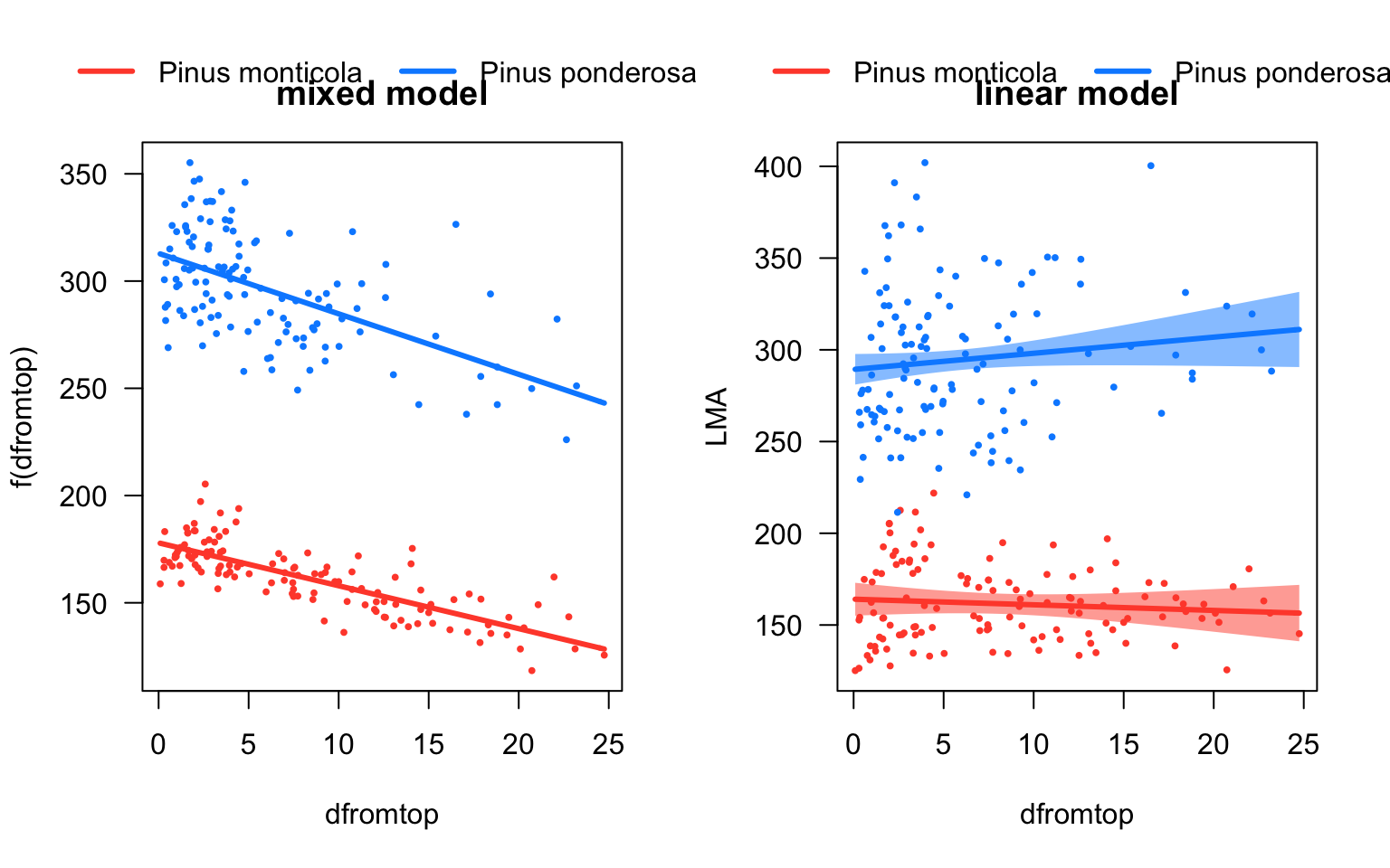
Ignoring the tree-to-tree variance thus resulted in drawing the wrong conclusion from our data. When we accounted for this variation with a mixed-effects model, we did find a significant overall relationship between LMA and dfromtop. The reason for this discrepancy is that the large variation in intercepts between the individual trees (between-subject variation) masked the relationship between the two variables within individuals (within-subject variation).
model diagnostics
plot(pref_m1)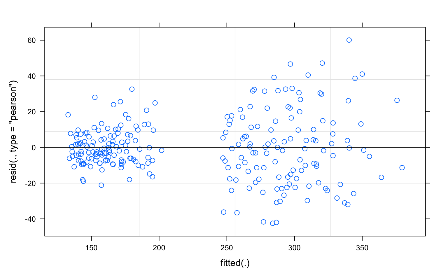
invisible(qqPlot(residuals(pref_m1)))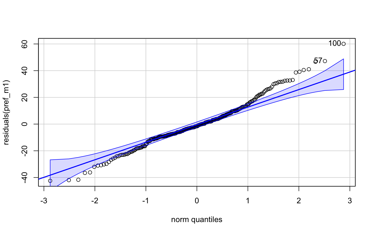
#The positive scaling of the residuals with increasing fitted values suggest that either a log- or square
# fit model with log-transformed response
pref_m2.ln <- lmer(log(LMA) ~ species + dfromtop + species:dfromtop +
                     (dfromtop|ID), data=pref)
# plot residuals against fitted values
plot(resid(pref_m2.ln) ~ fitted(pref_m2.ln))
abline(h=0)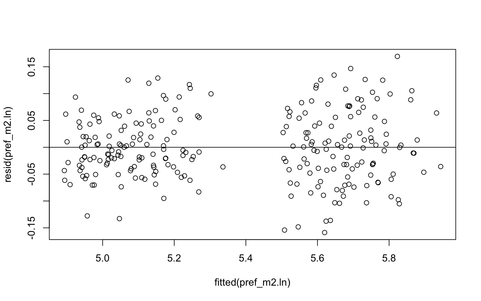
# quantile-quantile plot
invisible(qqPlot(residuals(pref_m2.ln)))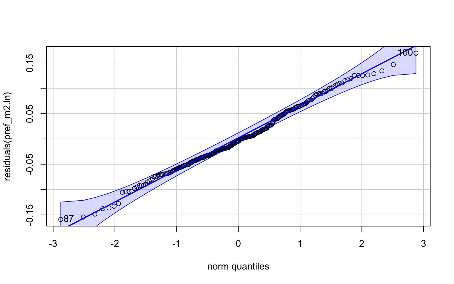
dataset2: individual-level variation in metabolic rate of mice
All example datasets used were download from hiercourse by Remko Duursma, Jeff Powell
data inspection
mouse <- read.csv("wildmousemetabolism.csv")
head(mouse)
## id run day temp food bm wheel rmr sex
## 1 99 1 1 31 No 14.11 No 0.02603748 Female
## 2 99 1 1 20 No 14.11 Yes 0.21428638 Female
## 3 99 1 1 15 No 14.11 Yes 0.12669190 Female
## 4 99 1 2 31 Yes 14.11 Yes 0.15794188 Female
## 5 99 1 2 20 Yes 14.11 Yes 0.22389830 Female
## 6 99 1 2 15 Yes 14.11 Yes 0.29547533 Female# Make sure the individual label ('id') is a factor variable
mouse$id <- as.factor(mouse$id)
length(unique(mouse$id))## [1] 16# looking at all rows for one mouse
# (not run, inspect yourself)
# that each mouse (id) was assessed at each of three temperatures (temp) over six consecutive days (day), and that this procedure was repeated three times (run).
# 3*6*3
dim(mouse[mouse$id == '99', ])## [1] 54 9# whether temperature has an effect on metabolic rate, and whether individuals were very different in terms of metabolic rate (rmr) at a fixed temperature.
par(mfrow=c(1,2))
with(mouse,plot(jitter(temp),rmr, pch=21, bg="#BEBEBE99", ylim=c(0,0.6)))
# Take a subset, and reorder the 'id' factor levels by rmr.
mouse15 <- subset(mouse, temp == 15)
mouse15$id <- with(mouse15, reorder(id, rmr, median, na.rm=TRUE))
# A simple boxplot showing variation in rmr across and within individuals
boxplot(rmr ~ id, data=mouse15, xlab="id", ylab="rmr",ylim=c(0,0.6))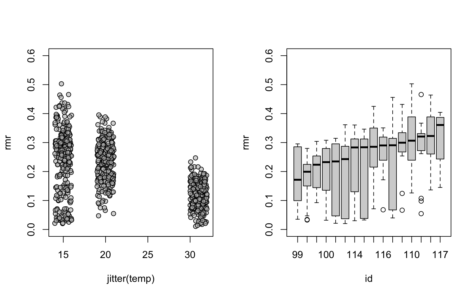
build mixed model, ‘run’ is nested within ‘id’
mouse_m0 <- lmer(rmr ~ temp + (1|id/run), data=mouse )
VarCorr(mouse_m0)
## Groups Name Std.Dev.
## run:id (Intercept) 0.029825
## id (Intercept) 0.027776
## Residual 0.071433#This demonstrates that the variation between individuals (id) is in fact similar to variation between runs within individuals (run:id).
Anova(mouse_m0)## Analysis of Deviance Table (Type II Wald chisquare tests)
##
## Response: rmr
## Chisq Df Pr(>Chisq)
## temp 459.93 1 < 2.2e-16 ***
## ---
## Signif. codes: 0 '***' 0.001 '**' 0.01 '*' 0.05 '.' 0.1 ' ' 1mouse$temp31 <- mouse$temp - 31
mouse_m1 <- lmer(rmr ~ temp31 + (1|id/run), data=mouse )
AIC(mouse_m0,mouse_m1)## df AIC
## mouse_m0 5 -1921.32
## mouse_m1 5 -1921.32add one predictor as fixed effect and compare models with ‘KRmodcomp’
mouse$temp31 <- mouse$temp - 31
mouse_m2 <- lmer(rmr ~ temp31*bm + (1|id/run), data=mouse )
library(pbkrtest)
KRmodcomp(mouse_m2, mouse_m1) #random strucutre the same, choose how many fixed effects to invovle in the model
## large : rmr ~ temp31 * bm + (1 | id/run)
## small : rmr ~ temp31 + (1 | id/run)
## stat ndf ddf F.scaling p.value
## Ftest 13.424 2.000 57.769 0.98861 1.629e-05 ***
## ---
## Signif. codes: 0 '***' 0.001 '**' 0.01 '*' 0.05 '.' 0.1 ' ' 1use Anova to get pvalue for fixed effects
#The F-test shows that including body mass and its interaction with temperature significantly improves the overall fit of the model. This does not tell us which of the terms is significant, but the Anova shows that both the main effect and interaction are significant:
Anova(mouse_m2, test="F")
## Analysis of Deviance Table (Type II Wald F tests with Kenward-Roger df)
##
## Response: rmr
## F Df Df.res Pr(>F)
## temp31 465.240 1 784.03 < 2.2e-16 ***
## bm 17.137 1 22.55 0.000411 ***
## temp31:bm 10.021 1 784.03 0.001608 **
## ---
## Signif. codes: 0 '***' 0.001 '**' 0.01 '*' 0.05 '.' 0.1 ' ' 1#An interesting side effect of including body mass as a fixed effect is that the estimated variance of the id is now much smaller. This makes sense because body mass varies between individuals, and thus including it in the model reduces the individual-level variation after having accounted for body mass.
#Compare the standard deviation for id for the mouse_m2 model (see below) with that estimated for the mouse_m0 model above.
VarCorr(mouse_m1)## Groups Name Std.Dev.
## run:id (Intercept) 0.029825
## id (Intercept) 0.027776
## Residual 0.071433VarCorr(mouse_m2)## Groups Name Std.Dev.
## run:id (Intercept) 0.029872
## id (Intercept) 0.012096
## Residual 0.071025library(variancePartition)
calcVarPart(mouse_m1)## id run:id temp31 Residuals
## 0.08055016 0.09287512 0.29380889 0.53276584calcVarPart(mouse_m2)## id run:id temp31 bm temp31:bm Residuals
## 0.0153119063 0.0933895546 0.0006097724 0.0239556617 0.3387873035 0.5279458015test whether a more complex random effects structure is supported by the data
We fit two models and compare them with a likelihood ratio test (with anova).
# Like mouse_m2, but with random slope (temp31)
mouse_m3 <- lmer(rmr ~ temp31*bm + (temp31|id/run), data=mouse )
anova(mouse_m3, mouse_m2)
## Data: mouse
## Models:
## mouse_m2: rmr ~ temp31 * bm + (1 | id/run)
## mouse_m3: rmr ~ temp31 * bm + (temp31 | id/run)
## npar AIC BIC logLik deviance Chisq Df Pr(>Chisq)
## mouse_m2 7 -1962.4 -1929.3 988.2 -1976.4
## mouse_m3 11 -1981.4 -1929.4 1001.7 -2003.4 26.998 4 1.99e-05 ***
## ---
## Signif. codes: 0 '***' 0.001 '**' 0.01 '*' 0.05 '.' 0.1 ' ' 1#The test shows that the more complex model is better, providing evidence that individuals differ sub- stantially in their response to temperature.
ggplot(mouse,aes(x=temp31,y=rmr))+geom_point()+
facet_wrap(.~id)+theme_bw()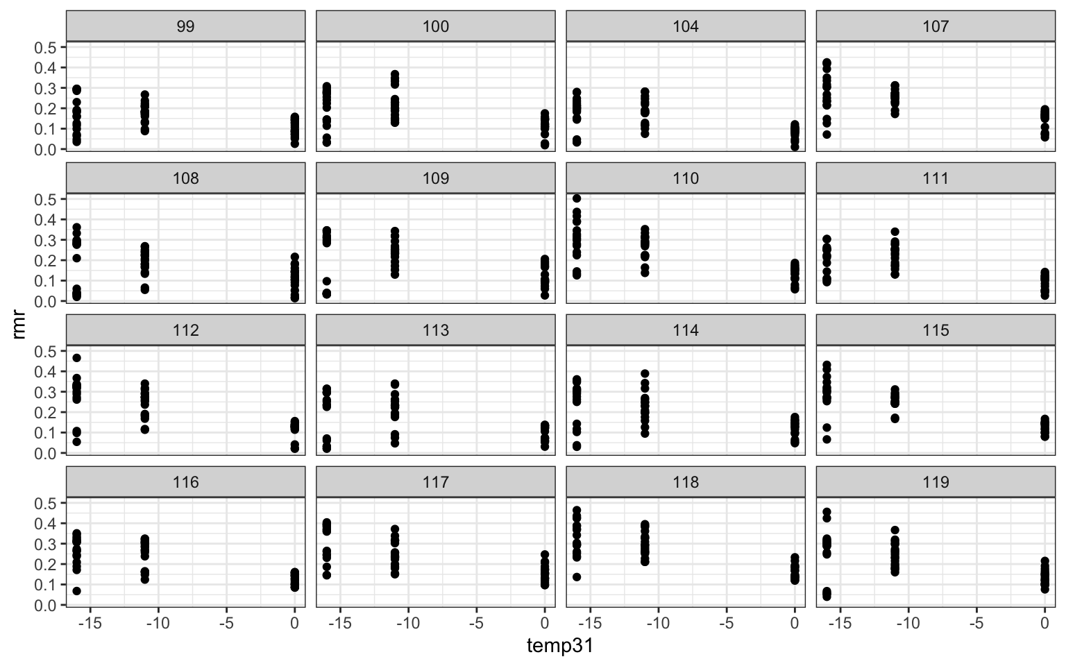
ggplot(mouse,aes(x=bm,y=rmr))+geom_point()+
  facet_wrap(.~id)+theme_bw()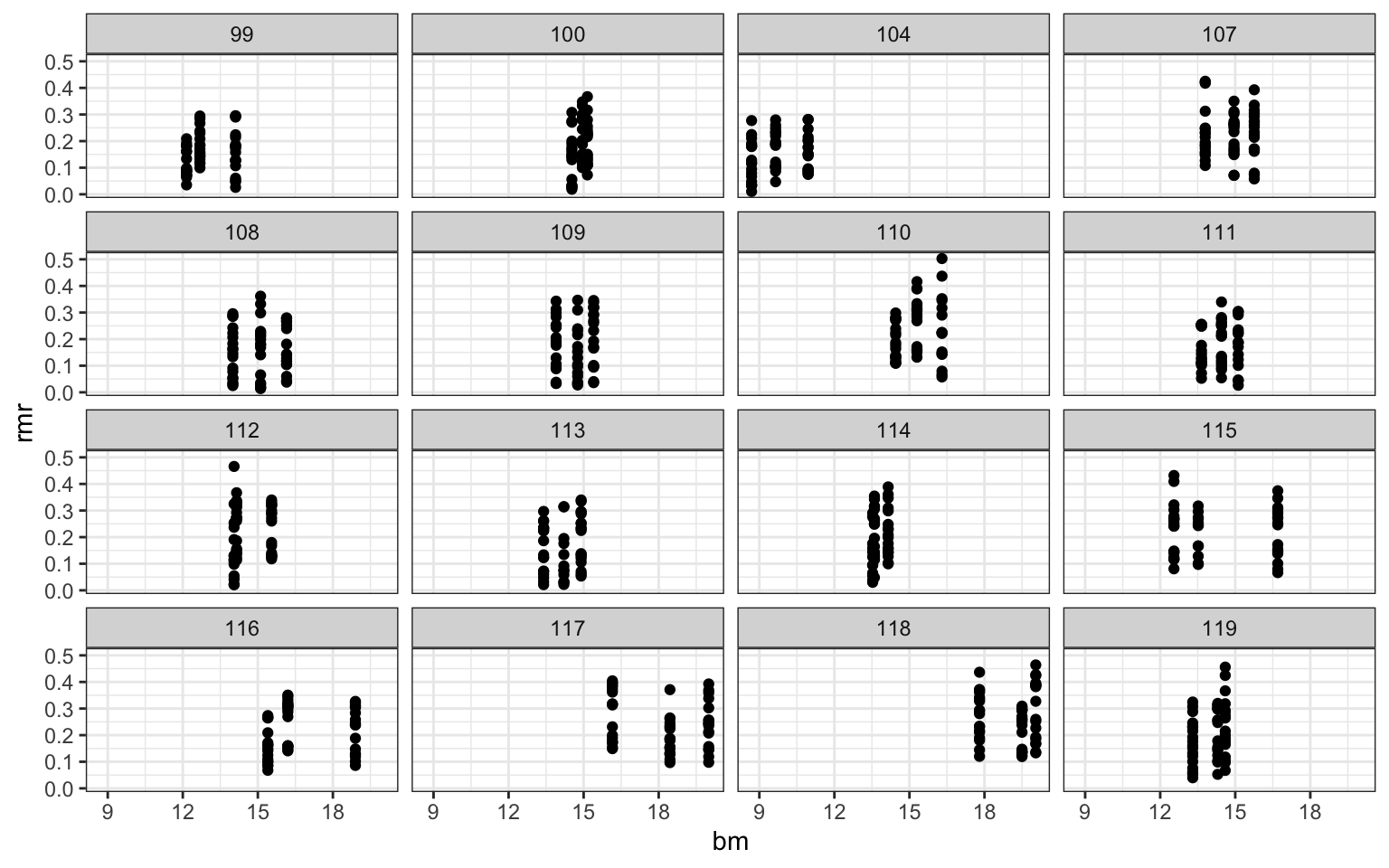
#As always, when we have a significant main effect and interaction, it is not easy to see how they affect the response variable. As always, it is most convenient to plot the model predictions with the visreg package. T
# Model predictions as a function of body mass, for the three temperatures.
# The argument 'partial=FALSE' turns off the partial residuals, producing a cleaner plot.
par(mfrow=c(1,2))
visreg(mouse_m3, "bm", by="temp31",overlay=TRUE, partial=FALSE, ylim=c(0,0.4))
visreg(mouse_m3, "bm", by="temp31",overlay=TRUE, partial=T, ylim=c(0,0.4))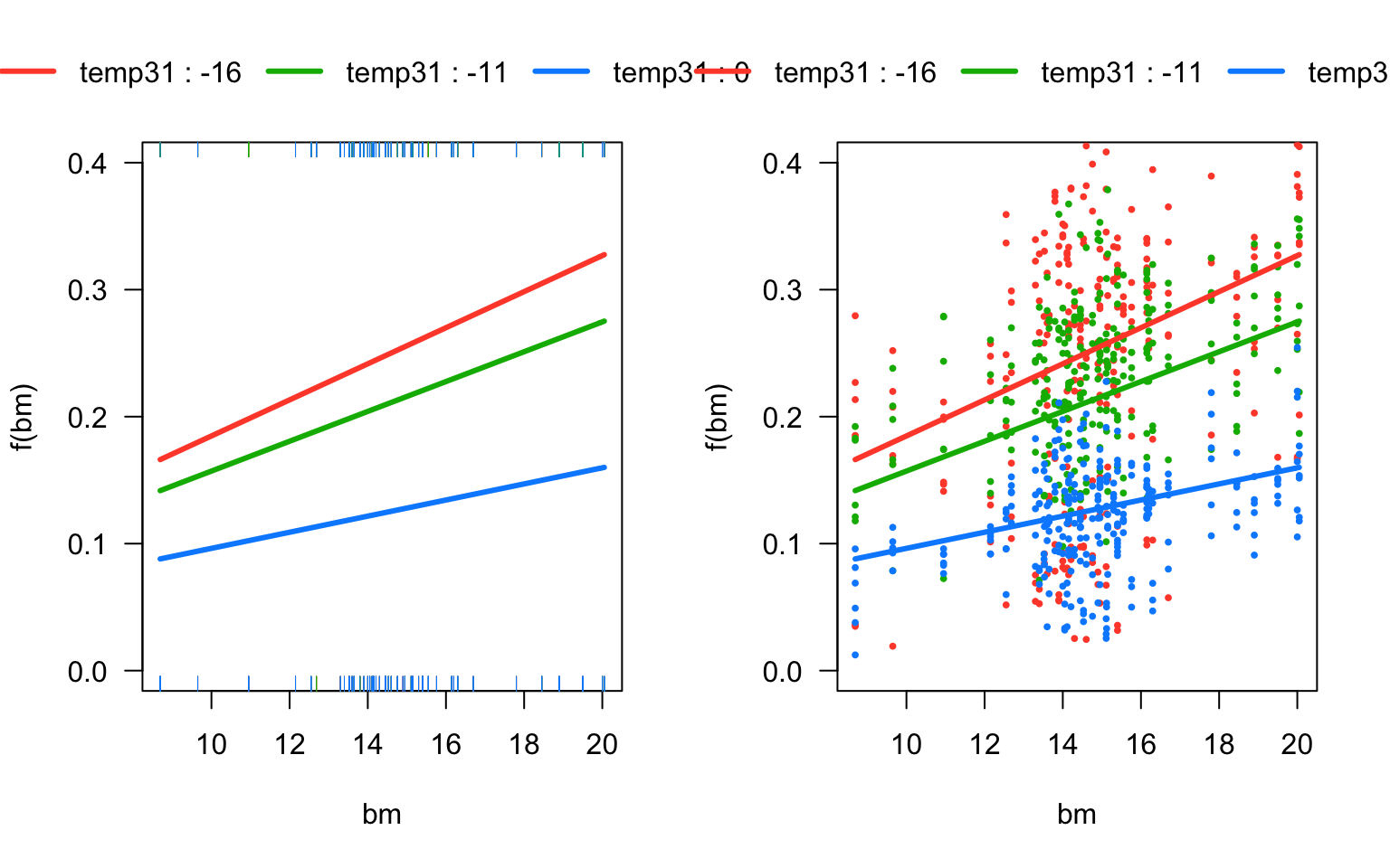
test for the effect of three additional fixed effects on metabolic rate.
As before, we test these effects one by one. The following code shows tests of sex and wheel on the rmr response variable.
# No effect of sex
mouse_m4 <- lmer(rmr ~ bm*temp31 + sex + (temp31|id/run), data=mouse)
KRmodcomp(mouse_m4, mouse_m3)
## large : rmr ~ bm * temp31 + sex + (temp31 | id/run)
## small : rmr ~ temp31 * bm + (temp31 | id/run)
## stat ndf ddf F.scaling p.value
## Ftest 0.2272 1.0000 16.1820 1 0.64# We add 'wheel' only as an additive effect. The interaction cannot be estimated because
# the only cases where 'wheel=No' were at a temperature of 31C:
with(mouse, table(temp,wheel))## wheel
## temp No Yes
## 15 0 288
## 20 0 288
## 31 144 144mouse_m5 <- lmer(rmr ~ bm*temp31 + wheel + (temp31|id/run), data=mouse)
KRmodcomp(mouse_m5, mouse_m3)## large : rmr ~ bm * temp31 + wheel + (temp31 | id/run)
## small : rmr ~ temp31 * bm + (temp31 | id/run)
## stat ndf ddf F.scaling p.value
## Ftest 46.546 1.000 740.235 1 1.862e-11 ***
## ---
## Signif. codes: 0 '***' 0.001 '**' 0.01 '*' 0.05 '.' 0.1 ' ' 1#We finish with the standard anova table, showing p-values for the main effects.
Anova(mouse_m5, test="F")## Analysis of Deviance Table (Type II Wald F tests with Kenward-Roger df)
##
## Response: rmr
## F Df Df.res Pr(>F)
## bm 11.9423 1 20.33 0.002453 **
## temp31 106.6980 1 22.30 5.776e-10 ***
## wheel 46.5458 1 740.23 1.862e-11 ***
## bm:temp31 4.3799 1 22.95 0.047619 *
## ---
## Signif. codes: 0 '***' 0.001 '**' 0.01 '*' 0.05 '.' 0.1 ' ' 1# Make a dataframe with all combinations of temp and id, for run 1 only
pred_dfr <- expand.grid(temp31=c(-16,-11,0),
id=levels(mouse$id), run=1)
# Get average body mass by individual, merge onto pred_dfr
library(doBy)
bmid <- summaryBy(bm ~ id, FUN=mean, data=mouse, keep.names=TRUE)
dim(bmid);dim(pred_dfr)## [1] 16 2## [1] 48 3pred_dfr <- merge(pred_dfr, bmid)
dim(pred_dfr)## [1] 48 4head(pred_dfr)## id temp31 run bm
## 1 100 -16 1 14.876667
## 2 100 -11 1 14.876667
## 3 100 0 1 14.876667
## 4 104 -16 1 9.763333
## 5 104 -11 1 9.763333
## 6 104 0 1 9.763333fixef(mouse_m3)## (Intercept) temp31 bm temp31:bm
## 0.0328485257 -0.0006177392 0.0063430582 -0.0004914050names(ranef(mouse_m3))## [1] "run:id" "id"# Predict rmr for every id and temp, from the mouse_m3 model
# The default behaviour is to make predictions including the random
# effects (i.e. id and run:id)
pred_dfr$rmr_pred <- predict(mouse_m3, pred_dfr)
# Plot the data for run 1
with(subset(mouse, run==1), plot(jitter(temp),rmr, pch=21, bg="#BEBEBE99", ylim=c(0,0.6)))
# Add a prediction line for every individual. This is an alternative implementation,
# avoiding a for loop. The use of invisible() avoids lapply from printing output.
invisible(lapply(split(pred_dfr, pred_dfr$id), function(x)lines(x$temp31 + 31, x$rmr_pred)))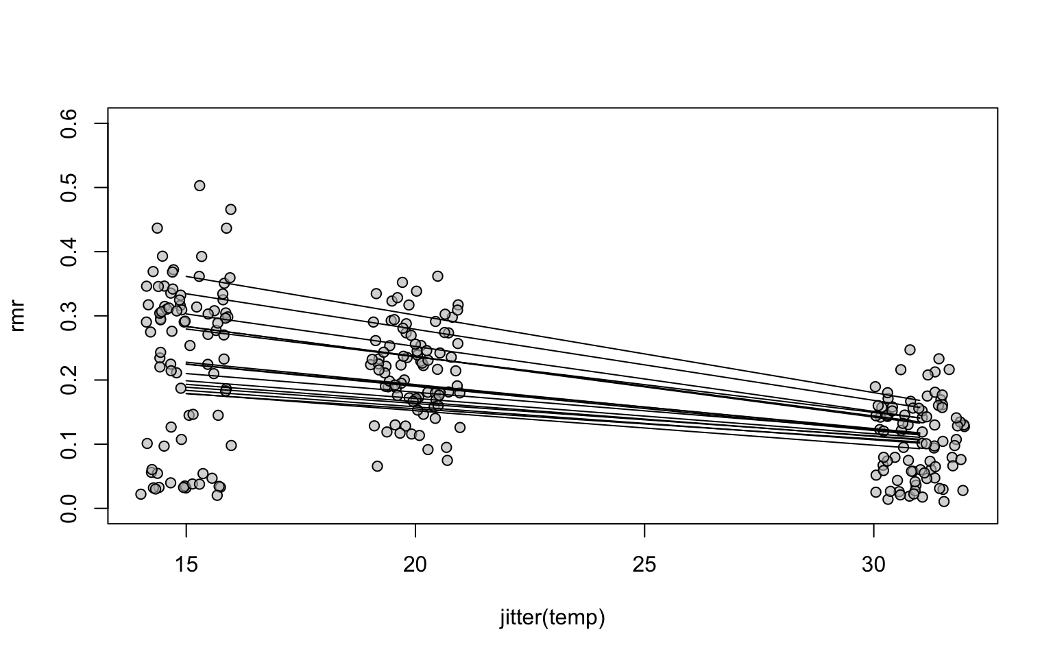
dataset3: blocked designs in the litter decomposition data
data inspection
litter <- read.csv("masslost.csv")
# Make sure the intended random effects (plot and block) are factors
litter$plot <- as.factor(litter$plot)
litter$block <- as.factor(litter$block)
litter$herbicide <- as.factor(litter$herbicide)
litter$profile <- as.factor(litter$profile)
head(litter)
## plot block variety herbicide profile date sample masslost
## 1 101 1 gm gly buried 07/18/06 incrop1 0.145
## 2 101 1 gm gly buried 07/18/06 incrop1 0.331
## 3 101 1 gm gly buried 07/18/06 incrop1 0.327
## 4 101 1 gm gly surface 07/18/06 incrop1 -0.102
## 5 101 1 gm gly surface 07/18/06 incrop1 -0.019
## 6 101 1 gm gly surface 07/18/06 incrop1 -0.046# Represent date as number of days since the start of the experiment
library(lubridate)
litter$date <- mdy(litter$date)
litter$date2 <- litter$date - ymd("2006-05-23")
# Quickly visualize the data to look for treatment effects
library(lattice)
bwplot(masslost ~ factor(date) | profile:herbicide, data=litter)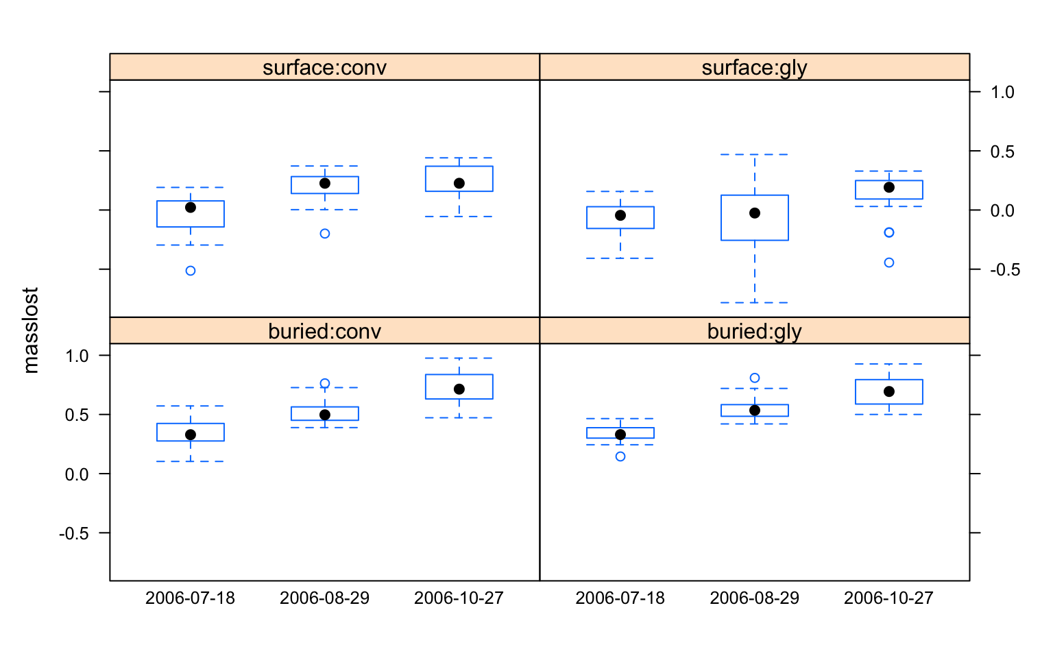
#We first fit a simple linear model which ignores some details of the experimental design, and use block as a fixed effect. It is often very useful to start with a linear model, perhaps on subsets of the data, to gradually try to make sense of the data.
# Count the data to confirm that the design is unbalanced (ignore blocks for brevity)
ftable(xtabs(~ date2 + profile + herbicide, data=litter))
## herbicide conv gly
## date2 profile
## 56 buried 22 22
## surface 21 21
## 98 buried 23 23
## surface 20 20
## 157 buried 19 16
## surface 18 21# Simple linear model with 'herbicide' as the first predictor in the model,
m1fix <- lm(masslost ~ date2 + herbicide * profile + block, data = litter)
Anova(m1fix)## Anova Table (Type II tests)
##
## Response: masslost
## Sum Sq Df F value Pr(>F)
## date2 3.7056 1 142.6601 < 2.2e-16 ***
## herbicide 0.3330 1 12.8198 0.0004157 ***
## profile 13.6594 1 525.8732 < 2.2e-16 ***
## block 0.4933 3 6.3311 0.0003793 ***
## herbicide:profile 0.3207 1 12.3475 0.0005284 ***
## Residuals 6.1820 238
## ---
## Signif. codes: 0 '***' 0.001 '**' 0.01 '*' 0.05 '.' 0.1 ' ' 1# fit model with random effects, plots nested within blocks
litter_m1 <- lmer(masslost ~ date2 + herbicide * profile + (1|block/plot),data = litter)
VarCorr(litter_m1) ## Groups Name Std.Dev.
## plot:block (Intercept) 0.000000
## block (Intercept) 0.047726
## Residual 0.161169# refit model without 'plot'
litter_m2 <- lmer(masslost ~ date2 + herbicide * profile + (1|block),data = litter)
anova(litter_m1, litter_m2)## Data: litter
## Models:
## litter_m2: masslost ~ date2 + herbicide * profile + (1 | block)
## litter_m1: masslost ~ date2 + herbicide * profile + (1 | block/plot)
## npar AIC BIC logLik deviance Chisq Df Pr(>Chisq)
## litter_m2 7 -183.7 -159.16 98.848 -197.7
## litter_m1 8 -181.7 -153.65 98.848 -197.7 0 1 1# look at significance of main effects and interactions
Anova(litter_m2, test="F")## Analysis of Deviance Table (Type II Wald F tests with Kenward-Roger df)
##
## Response: masslost
## F Df Df.res Pr(>F)
## date2 142.509 1 238.04 < 2.2e-16 ***
## herbicide 12.746 1 238.03 0.0004315 ***
## profile 526.217 1 238.03 < 2.2e-16 ***
## herbicide:profile 12.184 1 238.09 0.0005743 ***
## ---
## Signif. codes: 0 '***' 0.001 '**' 0.01 '*' 0.05 '.' 0.1 ' ' 1par(mfrow=c(1,2))
# Because we have three fixed effects, we can make two plots to visualize
# certain pairs of combinations.
visreg(litter_m2, "date2", by="profile",
ylab='mass lost (proportion)', overlay=TRUE)
visreg(litter_m2, "profile", by="herbicide", cond=list(date2=100),
ylab='mass lost (proportion)', overlay=TRUE)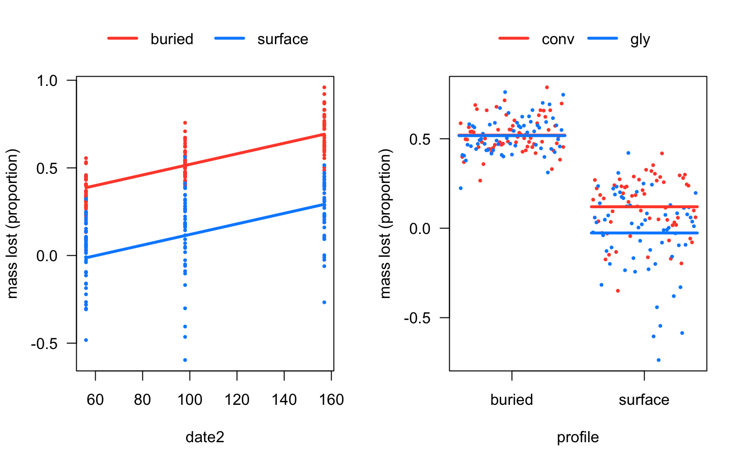
three ways to evaluate the importance of a term
# remove the interaction term from the model
litter_m2.int <- lmer(masslost ~ date2 + herbicide + profile + (1|block), data = litter)
# 1. anova
# Note that anova() will refit the models with ML (not REML) automatically,
# this is necessary when comparing models with different fixed or random effects terms.
anova(litter_m2, litter_m2.int)
## Data: litter
## Models:
## litter_m2.int: masslost ~ date2 + herbicide + profile + (1 | block)
## litter_m2: masslost ~ date2 + herbicide * profile + (1 | block)
## npar AIC BIC logLik deviance Chisq Df Pr(>Chisq)
## litter_m2.int 6 -173.68 -152.64 92.838 -185.68
## litter_m2 7 -183.70 -159.16 98.848 -197.70 12.02 1 0.0005263 ***
## ---
## Signif. codes: 0 '***' 0.001 '**' 0.01 '*' 0.05 '.' 0.1 ' ' 1# 2. KRmodcomp
library(pbkrtest)
KRmodcomp(litter_m2, litter_m2.int)## large : masslost ~ date2 + herbicide * profile + (1 | block)
## small : masslost ~ date2 + herbicide + profile + (1 | block)
## stat ndf ddf F.scaling p.value
## Ftest 12.184 1.000 238.087 1 0.0005743 ***
## ---
## Signif. codes: 0 '***' 0.001 '**' 0.01 '*' 0.05 '.' 0.1 ' ' 1# 3. AIC
AIC(litter_m2, litter_m2.int)## df AIC
## litter_m2 7 -146.9159
## litter_m2.int 6 -141.5371