log-log plot is “just” a way to “squeeze” the plot
In a log-log plot,
we are seeing the relationship between log(x) and log(y)
# polynomial, generate some data
x<-1:10; y=x*x
# Simple graph
plot(x, y)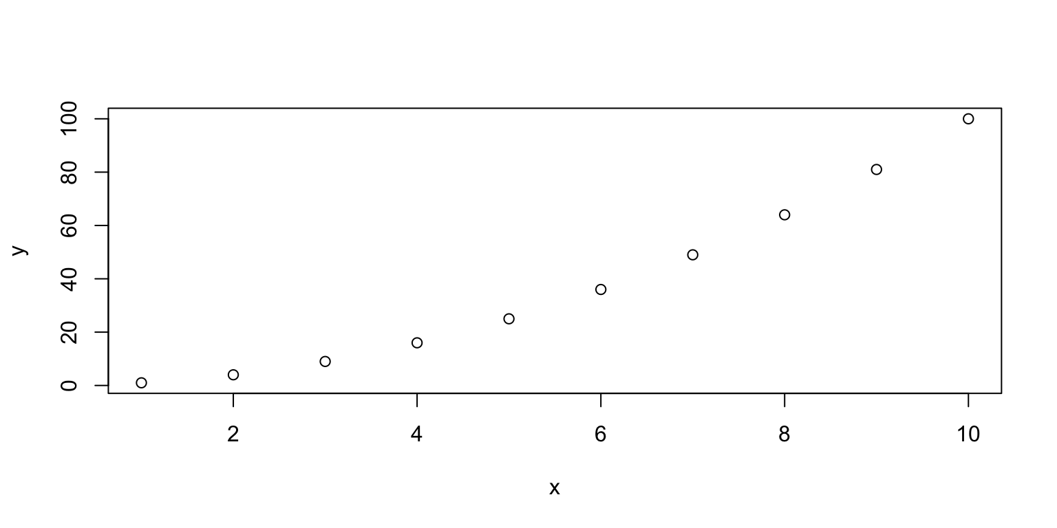
# Log on y-scale alone
par(mfrow=c(1,2),mar=c(5,4,2,1))
plot(x, y, log="y")
plot(x,log(y))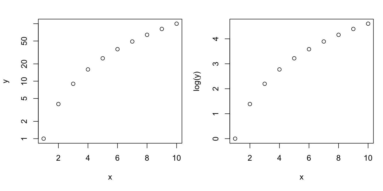
# distribution shapes are the same, just y-axis labeled differently.

# Log both axises
plot(x,y,log="xy")
plot(log(x),log(y))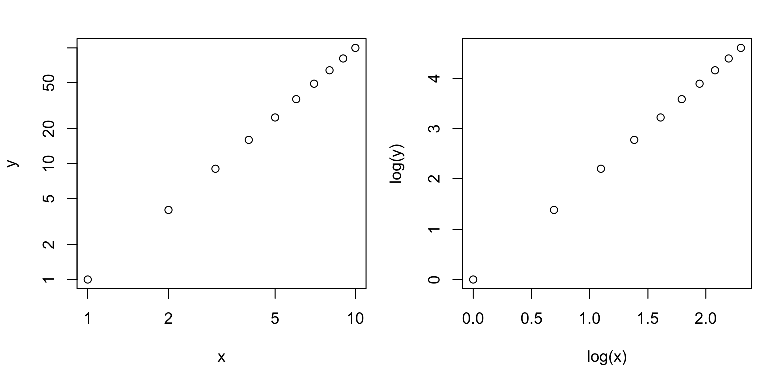
Why it is a straight line?
Remember we are looking at log(x) and log(y) on the log-log plot.
Let’s rephrase \(y = x^{2}\) by taking logarithm on both sides:
\(log(y) = 2 * log(x)\)
So, exactly, we expect to see a straight line with intercept 0 and slope 2.
Let’s try fit a regression line and check the slope.
but you could fit simple linear regression lines now!
new.y=log(y)
new.x=log(x)
out<-lm(new.y~new.x)
out
##
## Call:
## lm(formula = new.y ~ new.x)
##
## Coefficients:
## (Intercept) new.x
## -1.123e-15 2.000e+00plot(log(x),log(y))
abline(out)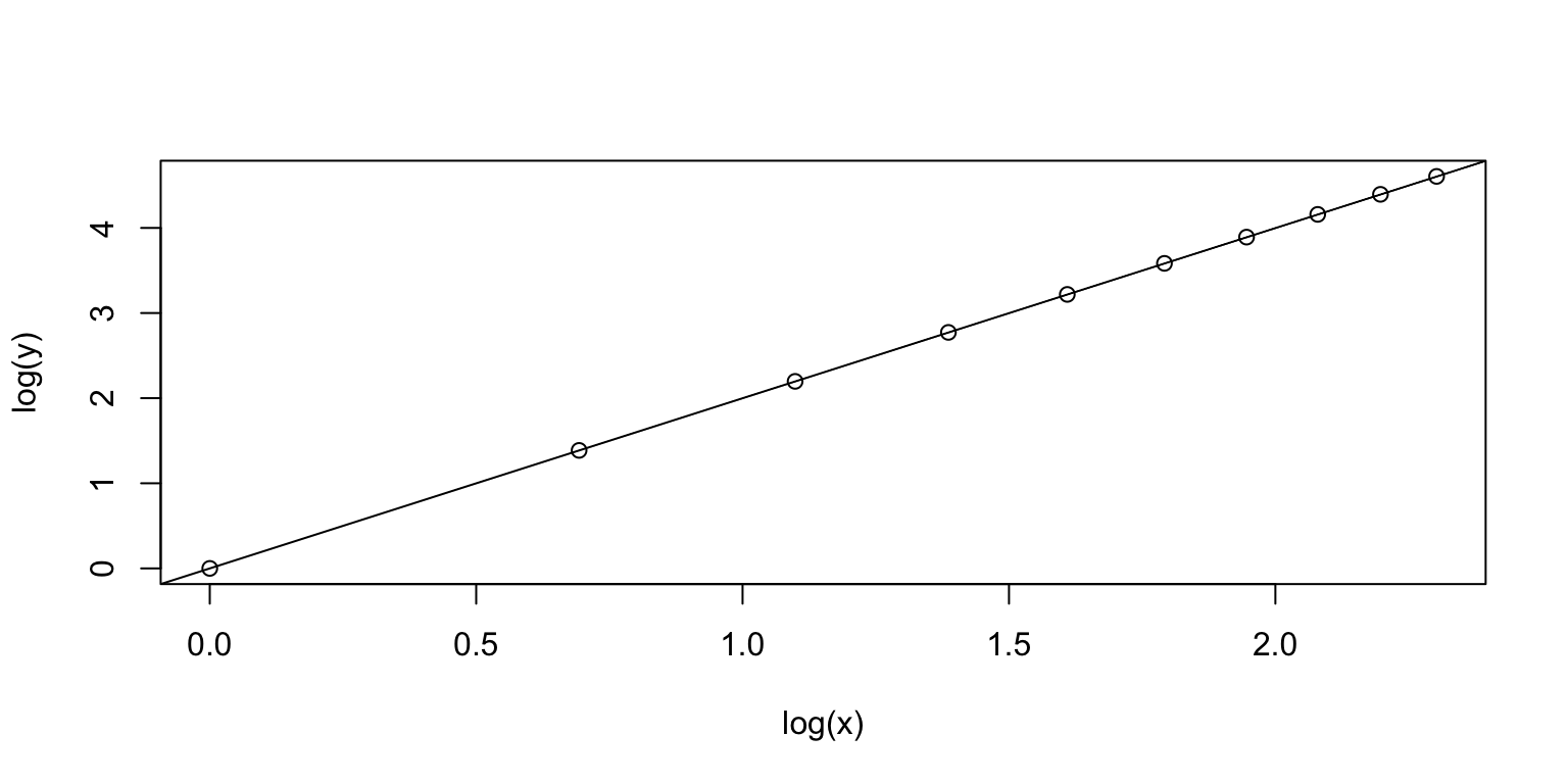
have fun with exponential distribution
\(f(x) = a*e^{-bx}\)
\(log(f(x)) = log(a) - bx\)
Let’s make thelog-log plot and see if there is a linear relationship.
# exponential, generate some data
a=3;
b=2;
x=1:10
y=a*exp(-b*x)
par(mfrow=c(1,3))
plot(x,y)
plot(x,y,log='xy')
plot(log(x),log(y))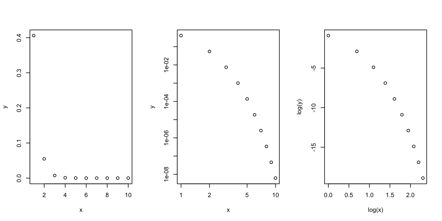
(out=lm(log(y)~log(x)))##
## Call:
## lm(formula = log(y) ~ log(x))
##
## Coefficients:
## (Intercept) log(x)
## 1.973 -7.861Wait…. The middle and rightmost plots do not look like a straight line.
What happened?
Remember, on a log-lot plot we are seeing the relationship between log(y) and log(x), NOT log(y) and x.
So what’s the relationship between log(y) and log(x) after all.
Let’s “play magic” on the equation.
While there is no explict log(x) in the above equation,
we can make it happen by the fact: \(x = exp^{log(x)}\),
then we have:
\(log(f(x)) = log(a) - b*exp^{log(x)}\)
So, it’s pretty clear we don’t have a linear relationship between log(x) and log(y).
Sad… but below is something fun!
Power Function and Power Law distribution
I won’t talk too much about the Power Law distribution as it’s too cheap and easy and cliche… It’s not cool!!!
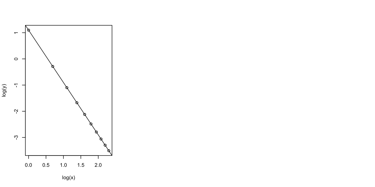
Just a snippet. \(y = Cx^{-a}\)
\(log(y) = log(C) - a*log(x)\)
C=3
a=2
x=1:10
y=C*x^(-a)
par(mfrow=c(1,3))
plot(x,y)
plot(x,y,log='xy')
plot(log(x),log(y))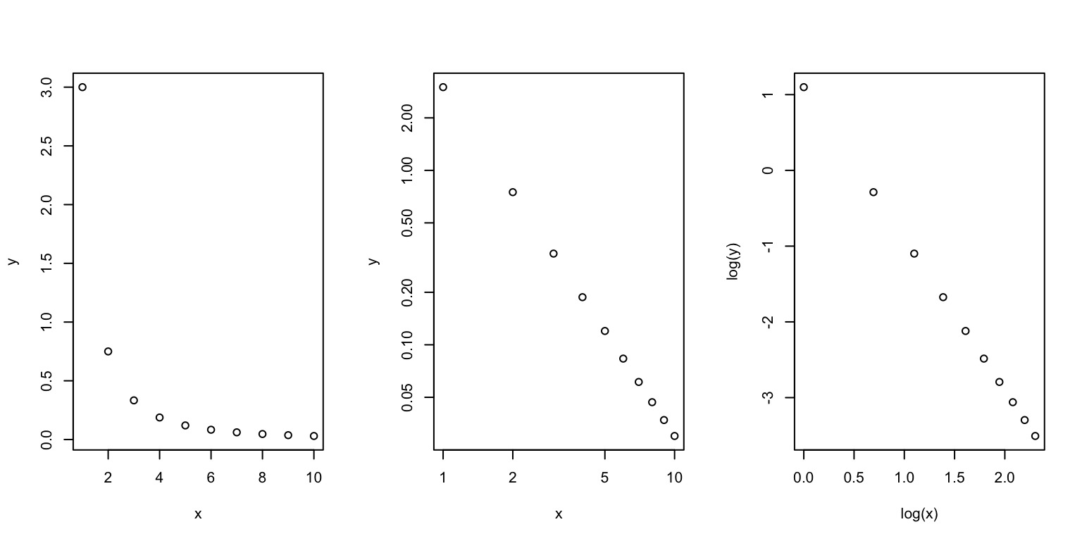
(out<-lm(log(y)~log(x)))##
## Call:
## lm(formula = log(y) ~ log(x))
##
## Coefficients:
## (Intercept) log(x)
## 1.099 -2.000log(C)## [1] 1.098612-a## [1] -2plot(log(x),log(y))
abline(out)