basic model
\(y = b0 + b1*x1 + b2*x2 + b3*(x1+x2)\)
Scenario 1: one numeric + one factor
load the data
library(tidyverse)
data(mtcars)
glimpse(mtcars)
## Rows: 32
## Columns: 11
## $ mpg <dbl> 21.0, 21.0, 22.8, 21.4, 18.7, 18.1, 14.3, 24.4, 22.8, 19.2, 17.8,…
## $ cyl <dbl> 6, 6, 4, 6, 8, 6, 8, 4, 4, 6, 6, 8, 8, 8, 8, 8, 8, 4, 4, 4, 4, 8,…
## $ disp <dbl> 160.0, 160.0, 108.0, 258.0, 360.0, 225.0, 360.0, 146.7, 140.8, 16…
## $ hp <dbl> 110, 110, 93, 110, 175, 105, 245, 62, 95, 123, 123, 180, 180, 180…
## $ drat <dbl> 3.90, 3.90, 3.85, 3.08, 3.15, 2.76, 3.21, 3.69, 3.92, 3.92, 3.92,…
## $ wt <dbl> 2.620, 2.875, 2.320, 3.215, 3.440, 3.460, 3.570, 3.190, 3.150, 3.…
## $ qsec <dbl> 16.46, 17.02, 18.61, 19.44, 17.02, 20.22, 15.84, 20.00, 22.90, 18…
## $ vs <dbl> 0, 0, 1, 1, 0, 1, 0, 1, 1, 1, 1, 0, 0, 0, 0, 0, 0, 1, 1, 1, 1, 0,…
## $ am <dbl> 1, 1, 1, 0, 0, 0, 0, 0, 0, 0, 0, 0, 0, 0, 0, 0, 0, 1, 1, 1, 0, 0,…
## $ gear <dbl> 4, 4, 4, 3, 3, 3, 3, 4, 4, 4, 4, 3, 3, 3, 3, 3, 3, 4, 4, 4, 3, 3,…
## $ carb <dbl> 4, 4, 1, 1, 2, 1, 4, 2, 2, 4, 4, 3, 3, 3, 4, 4, 4, 1, 2, 1, 1, 2,…# to start with, visualize each predictor effect separately
par(mfrow=c(1,2),mar=c(3,3,1,1))
plot(mtcars$disp,mtcars$mpg)
boxplot(mpg~vs,data=mtcars)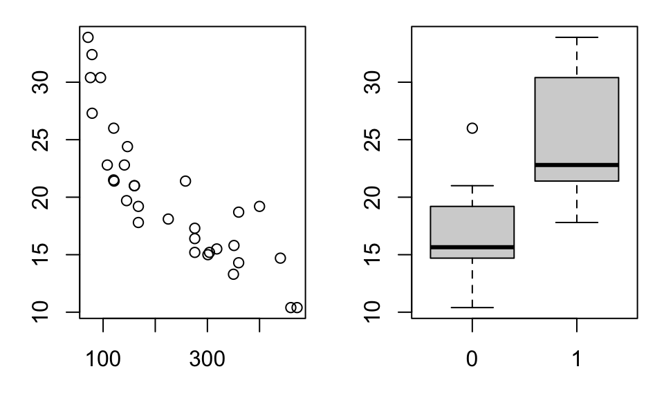
# try to have a holistic view
ggplot(data=mtcars,aes(x=disp,y=mpg))+geom_point()+facet_wrap(.~vs)+theme_bw(base_size = 15)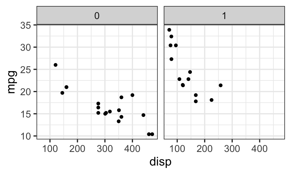
# make it even simple and clear
ggplot(data=mtcars,aes(x=disp,y=mpg,col=factor(vs)))+geom_point()+theme_bw(base_size = 15)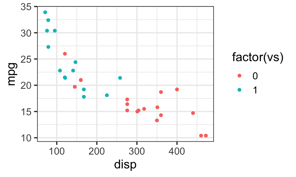
Asking ‘is there interaction between disp and vs’, is like asking: if I fit lines for green dots and red dots separately,
- would the two lines be the same?
- have different intercept?
- have different slopes?
build two linear models
m0<-lm(mpg~disp+vs,data=mtcars)
m1<-lm(mpg~disp*vs,data=mtcars)
anova(m0,m1)
## Analysis of Variance Table
##
## Model 1: mpg ~ disp + vs
## Model 2: mpg ~ disp * vs
## Res.Df RSS Df Sum of Sq F Pr(>F)
## 1 29 308.44
## 2 28 246.91 1 61.527 6.9772 0.01335 *
## ---
## Signif. codes: 0 '***' 0.001 '**' 0.01 '*' 0.05 '.' 0.1 ' ' 1The anova shows linear model with the interaction term, m1 in the above code, fits the data slightly better with a pvalue 0.01335.
Then how to interpret the m0 and m1 models?
As the basic linear model is: \(y = b0 + b1*x1 + b2*x2 + b3*(x1+x2)\)
in our case, x1=disp, x2=vs
interprete the model without interaction
for model m0: \(y = b0 + b1*disp + b2*vs\)
- vs=0, \(y = b0 + b1*disp\)
- vs=1, \(y = b0 + b1*disp + b2\)
or, \(y = b0 +b2 + b1*disp\)
Thus, without the interaction term, the effect of vs only show up for the intercept, which means there are two parallele lines for blue and red dots.
(x=coef(m0))## (Intercept) disp vs
## 27.94928175 -0.03689603 1.49500359ggplot(data=mtcars,aes(x=disp,y=mpg,col=factor(vs)))+geom_point()+theme_bw(base_size = 15)+
geom_abline(intercept = x[1], slope = x[2], color="#F8766D",
linetype="dashed", size=1)+
geom_abline(intercept = x[1]+x[3], slope = x[2], color="#00BFC4",
linetype="dashed", size=1)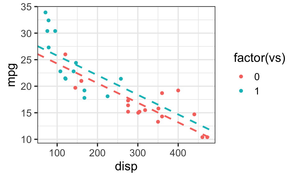
To interpret m0,
- holding
vsconstant, if increasedispby 100, thempgwould increase b1*100 = -3.6896028. - holding
dispconstant, cars withvs=1is b2 = 1.4950036 larger thanvs=0ones.
interprete the model with interaction
for model m1: \(y = b0 + b1*disp + b2*vs + b3*disp*vs\)
- vs=0, \(y = b0 + b1*disp\)
- vs=1, \(y = b0 + b1*disp + b2 + b3*disp\)
or, \(y = b0 +b2 + (b1+b3)*disp\)
Thus, with the interaction term, the effect of vs show up both for the intercept and the slope, which means the lines would intercross.
(x=coef(m1)) #b0,b1,b2,b3## (Intercept) disp vs disp:vs
## 25.63755459 -0.02936965 8.39770888 -0.04218648ggplot(data=mtcars,aes(x=disp,y=mpg,col=factor(vs)))+geom_point()+theme_bw(base_size = 15)+
geom_abline(intercept = x[1], slope = x[2], color="#F8766D",
linetype="dashed", size=1)+
geom_abline(intercept = x[1]+x[3], slope = x[2]+x[4], color="#00BFC4",
linetype="dashed", size=1)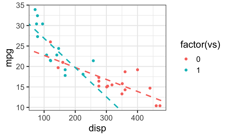
To interpret m1,
- holding
vsconstant, if increasedispby 100,- if
vs=0, thempgwould increase b1*100 = -2.936965. - if
vs=1, thempgwould increase (b1+b3)*100 = -7.1556131.
- if
- holding
dispconstant, cars withvs=1is b2+b3*disp = 8.3977089 + -0.0421865*disp larger thanvs=0ones.
Scenario 2: one factor + one factor
Basic linear model: \(y = b0 + b1*x1 + b2*x2 + b3*(x1+x2)\)
in this case, x1=am, x2=vs
# to start with, visualize each predictor effect separately
par(mfrow=c(1,2),mar=c(3,3,1,1))
boxplot(mpg~am,data=mtcars)
boxplot(mpg~vs,data=mtcars)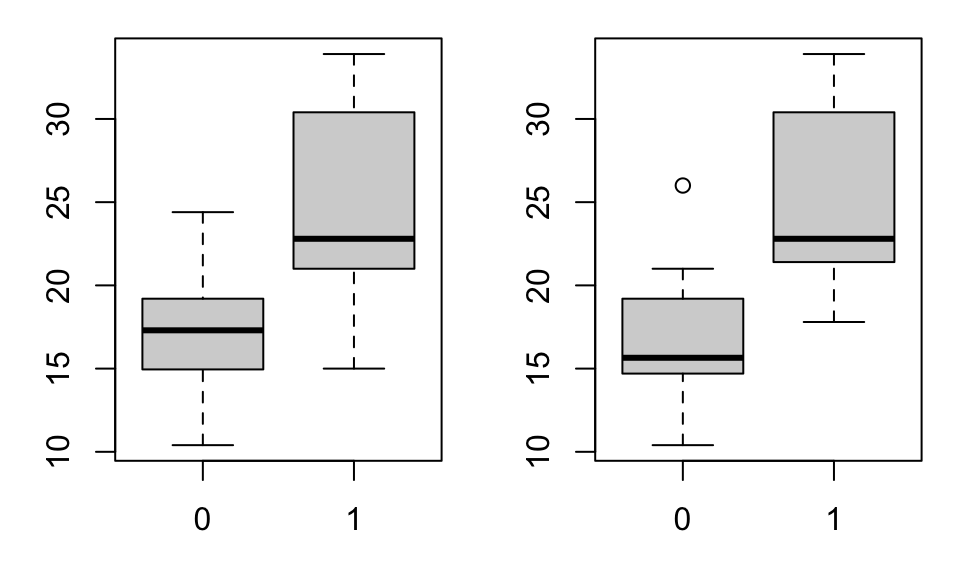
# try to have a holistic view
ggplot(data=mtcars,aes(x=factor(am),y=mpg))+geom_boxplot()+facet_wrap(.~vs)+theme_bw(base_size = 15)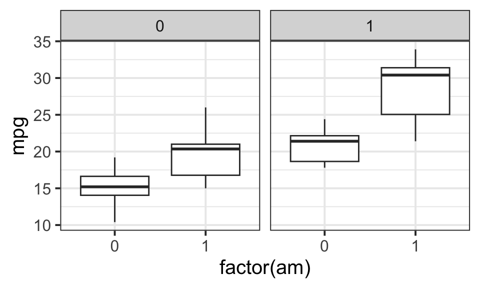
# make it even simple and clear
ggplot(data=mtcars,aes(x=factor(am),y=mpg,col=factor(vs)))+geom_boxplot()+theme_bw(base_size = 15)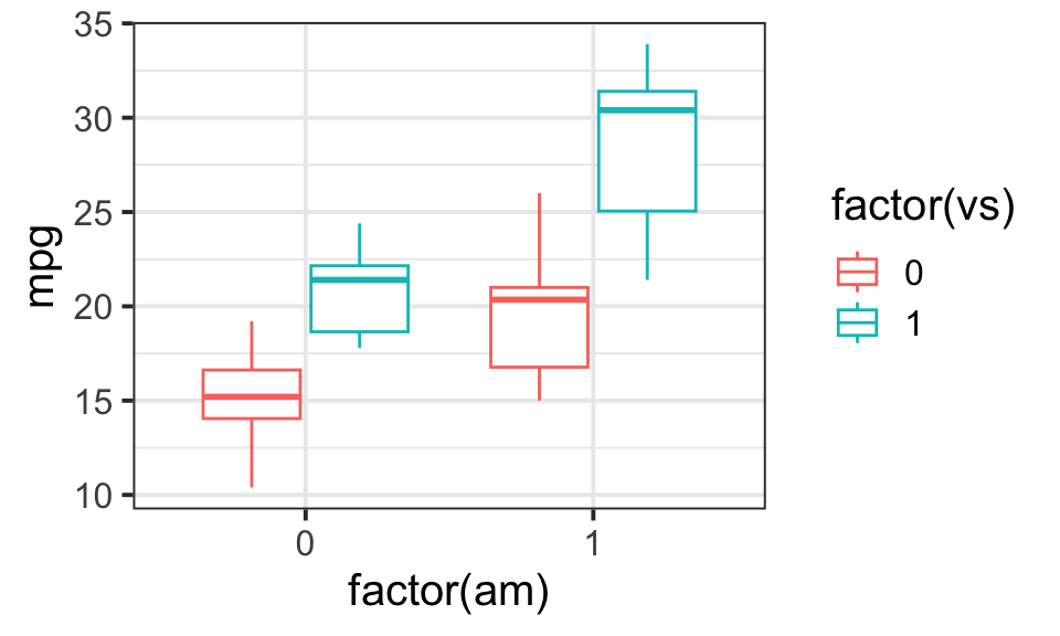
ggplot(data=mtcars,aes(x=factor(am),y=mpg,col=factor(vs)))+
  geom_line(aes(group=factor(vs)),position = position_dodge(width = 0.5))+geom_point(position = position_dodge(width = 0.5))+theme_bw(base_size = 15)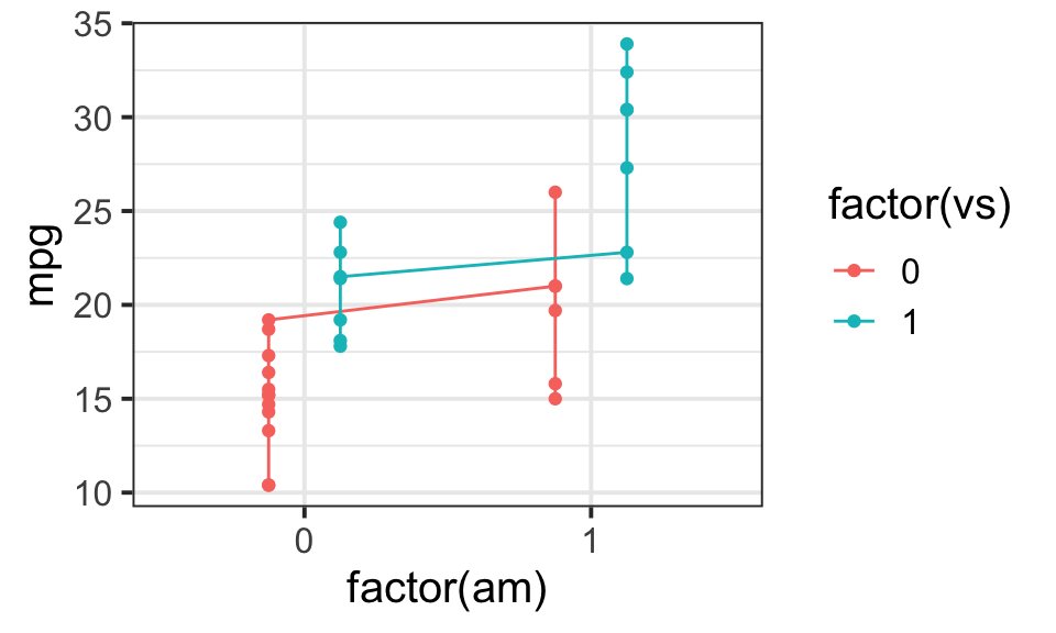
m0=lm(mpg~vs+am,data=mtcars)
m1=lm(mpg~vs*am,data=mtcars)
anova(m0,m1)
## Analysis of Variance Table
##
## Model 1: mpg ~ vs + am
## Model 2: mpg ~ vs * am
## Res.Df RSS Df Sum of Sq F Pr(>F)
## 1 29 353.49
## 2 28 337.48 1 16.009 1.3283 0.2589without interaction \(y = b0 + b1*am + b2*vs\)
- vs=0, \(y = b0 + b1*am\)
- vs=1, \(y = b0 + b2 + b1*am\)
Similarly,
- am=0, \(y = b0 + b2*vs\)
- am=1, \(y = b0 + b1 + b2*vs\)
The effect of am or vs does not depend on the other term.
- Holding
vsconstant, increase of 100amlead to b1*100 increase inmpg. - Holding
amconstant, increase of 100vslead to b2*100 increase inmpg.
with interaction \(y = b0 + b1*am + b2*vs + b3*am*vs\)
- vs=0, \(y = b0 + b1*am\)
- vs=1, \(y = b0 + b2 + (b1+b3)*am\)
Similarly,
- am=0, \(y = b0 + b2*vs\)
- am=1, \(y = b0 + b1 + (b2+b3)*vs\)
Factors of am or vs affect each other.
- Holding
vsconstant, increase of 100amlead to (b1+b3)*100 increase inmpg. - Holding
amconstant, increase of 100vslead to (b2+b3)*100 increase inmpg.
Scenario 3: one numeric + one numeric
# to start with, visualize each predictor effect separately
par(mfrow=c(1,2),mar=c(3,3,1,1))
plot(mpg~disp,data=mtcars)
plot(mpg~drat,data=mtcars)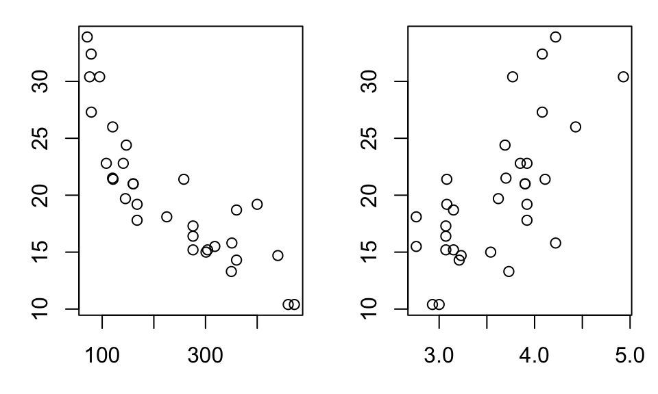
# try to have a holistic view, as it's two numeric predictor,
# there is no easy to visualize them
ggplot(data=mtcars,aes(x=disp,y=mpg,col=drat))+geom_point()+theme_bw(base_size = 15)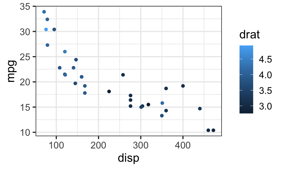
m0=lm(mpg~disp+drat,data=mtcars)
m1=lm(mpg~disp*drat,data=mtcars)
anova(m0,m1)
## Analysis of Variance Table
##
## Model 1: mpg ~ disp + drat
## Model 2: mpg ~ disp * drat
## Res.Df RSS Df Sum of Sq F Pr(>F)
## 1 29 302.90
## 2 28 246.88 1 56.02 6.3537 0.01769 *
## ---
## Signif. codes: 0 '***' 0.001 '**' 0.01 '*' 0.05 '.' 0.1 ' ' 1interprete the model without interaction
without interaction \(y = b0 + b1*disp + b2*drat\)
The effect of disp or drat does not depend on the other term.
- Holding
dratconstant, increase of 100displead to b1*100 increase inmpg. - Holding
dispconstant, increase of 100dratlead to b2*100 increase inmpg.
(x=coef(m0))## (Intercept) disp drat
## 21.84487993 -0.03569388 1.80202739g1<-ggplot(data=mtcars,aes(x=disp,y=mpg))+geom_point()+theme_bw(base_size = 15)+xlim(c(0,500))+
geom_abline(intercept = x[1], slope = x[2], color="#F8766D",
linetype="dashed", size=1)
g2<-ggplot(data=mtcars,aes(x=drat,y=mpg))+geom_point()+theme_bw(base_size = 15)+xlim(c(0,5))+
geom_abline(intercept = x[1], slope = x[3], color="#00BFC4",
linetype="dashed", size=1)
gridExtra::grid.arrange(g1,g2,ncol=2)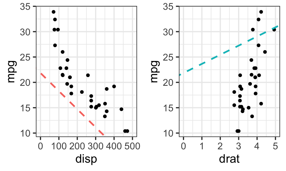
interprete the model with interaction
without interaction \(y = b0 + b1*disp + b2*drat + b3*disp*drat\)
The effect of disp or drat depends on the other term.
- Holding
dratconstant, increase of 100displead to (b1+b3*drat)*100 increase inmpg. - Holding
dispconstant, increase of 100dratlead to (b2+b3*disp)*100 increase inmpg.
Some useful ref
https://ademos.people.uic.edu/Chapter13.html#2_continuous_x_continuous_regression