A predictor/response variable could be either numeric or factor.
When the response variable is a continuous numeric,
- ANOVA: the predictors are factors.
- regression: the predictors are continuous numeric values.
- linear model: a mix of factors and continuous predictors.
- when there is one continuous variable and one factor variable, it’s called ANCOVA (analysis of covariance).
- mixed models: the factors are for grouping and account for non-independent relationship between observations.
When the response variable is a binary number or non-negative integers,
- glm: Generalized Linear Models
get overall model pvalue
- All example datasets used below were download from hiercourse by Remko Duursma, Jeff Powell
coweeta<-read.csv("coweeta.csv")

# Take a subset and drop empty levels with droplevels.
cowsub <- droplevels(subset(coweeta, species %in% c("cofl","bele","oxar","quru")))

# Quick summary table
with(cowsub, tapply(height, species, mean))
## bele cofl oxar quru
## 21.86700 6.79750 16.50500 21.10556boxplot(height~species,data=cowsub)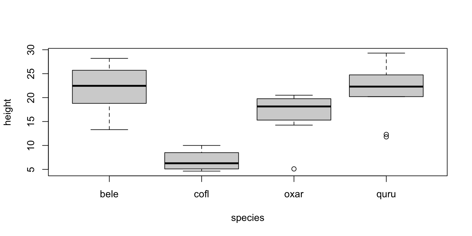
fit1 <- lm(height ~ species, data=cowsub)
fit1
##
## Call:
## lm(formula = height ~ species, data = cowsub)
##
## Coefficients:
## (Intercept) speciescofl speciesoxar speciesquru
## 21.8670 -15.0695 -5.3620 -0.7614summary(fit1)##
## Call:
## lm(formula = height ~ species, data = cowsub)
##
## Residuals:
## Min 1Q Median 3Q Max
## -11.405 -2.062 0.695 3.299 8.194
##
## Coefficients:
## Estimate Std. Error t value Pr(>|t|)
## (Intercept) 21.8670 1.5645 13.977 7.02e-14 ***
## speciescofl -15.0695 2.9268 -5.149 2.04e-05 ***
## speciesoxar -5.3620 2.3467 -2.285 0.0304 *
## speciesquru -0.7614 2.2731 -0.335 0.7402
## ---
## Signif. codes: 0 '***' 0.001 '**' 0.01 '*' 0.05 '.' 0.1 ' ' 1
##
## Residual standard error: 4.947 on 27 degrees of freedom
## Multiple R-squared: 0.5326, Adjusted R-squared: 0.4807
## F-statistic: 10.26 on 3 and 27 DF, p-value: 0.0001111Two things about the summary() output:
a t-statistic for each coefficient, and p-value for testing the deviation against zero. Not surprisingly the Intercept (i.e., the mean for the first species) is significantly different from zero (as indicated by the very small p-value). Two of the next three coefficients are also significantly different from zero.
At the end of the summary, the F-statistic and corresponding p-value are shown. This p-value tells us whether the whole model is significant. In this case, it is comparing a model with four coefficients (one for each species) to a model that just has the same mean for all groups. In this case, the model is highly significant – i.e. there is evidence of different means for each group. In other words, a model where the mean varies between the four species performs much better than a model with a single grand mean.
pairwise level comparison within a factor predictor
The ANOVA above gives a single p-value for the overall ‘species effect’, and whether individual species are different from the first level in the model.
To get whether the four species are all different from each other, below shows a multiple comparison test.
lmSpec<-lm(height~species,data=cowsub)
library(emmeans)
# Estimate marginal means and confidence interval for each level of 'species'.
tukey_Spec<-emmeans(lmSpec,'species')
summary(tukey_Spec)
## species emmean SE df lower.CL upper.CL
## bele 21.9 1.56 27 18.66 25.1
## cofl 6.8 2.47 27 1.72 11.9
## oxar 16.5 1.75 27 12.92 20.1
## quru 21.1 1.65 27 17.72 24.5
##
## Confidence level used: 0.95# Print results of contrasts. This shows p-values for the null hypotheses
# that species A is no different from species B, and so on.
pairs(tukey_Spec,adjust='bonferroni') #the p-values are adjusted for multiple comparisons ## contrast estimate SE df t.ratio p.value
## bele - cofl 15.069 2.93 27 5.149 0.0001
## bele - oxar 5.362 2.35 27 2.285 0.1824
## bele - quru 0.761 2.27 27 0.335 1.0000
## cofl - oxar -9.707 3.03 27 -3.204 0.0208
## cofl - quru -14.308 2.97 27 -4.813 0.0003
## oxar - quru -4.601 2.40 27 -1.914 0.3978
##
## P value adjustment: bonferroni method for 6 testspwpp(tukey_Spec)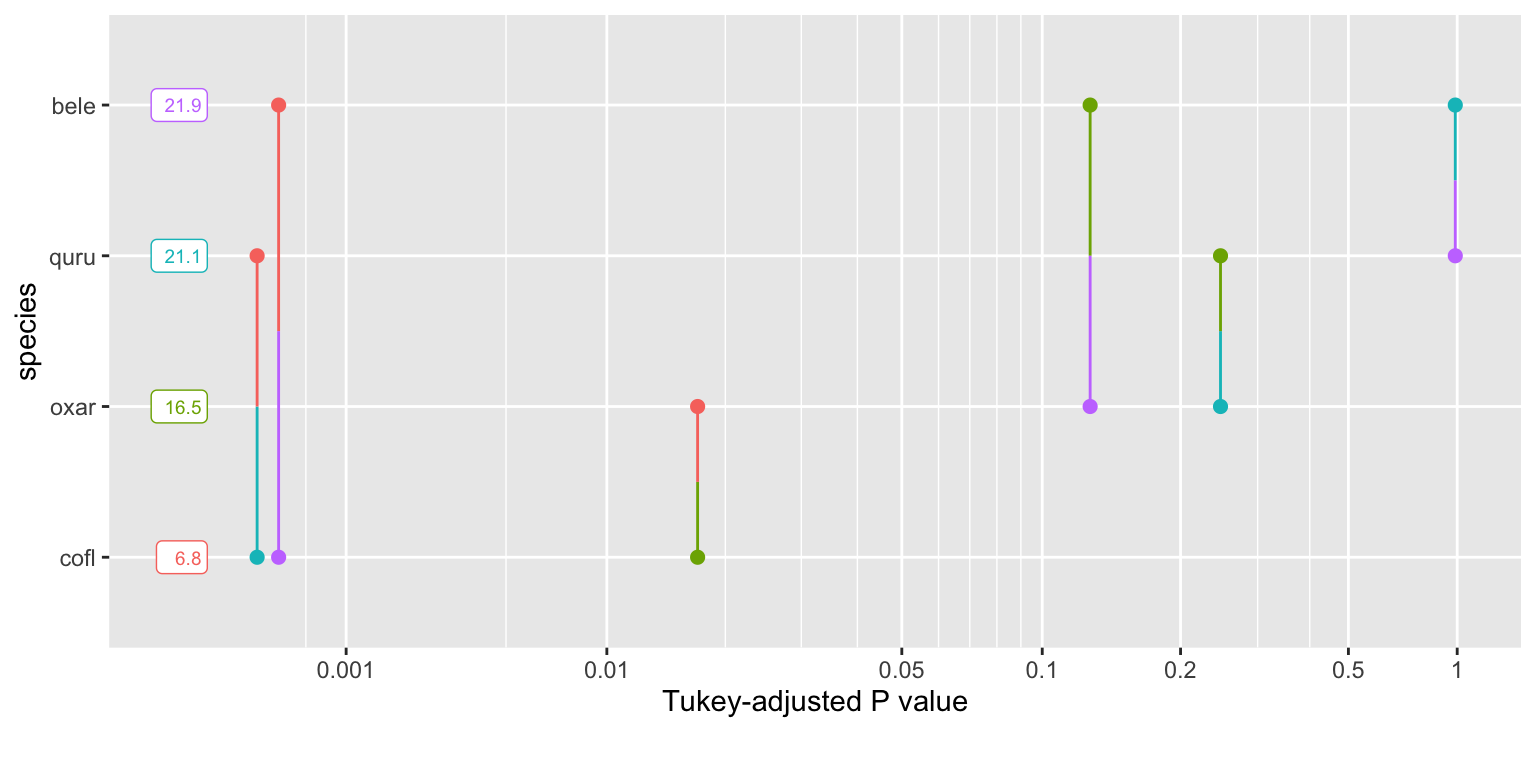
significance of individual factor when there are multiple predictors
play with two factor predictors
memory <- read.table("eysenck.txt", header=TRUE)
# Count nr of observations
xtabs( ~ Age + Process, data=memory)
## Process
## Age Adjective Counting Imagery Intentional Rhyming
## Older 10 10 10 10 10
## Younger 10 10 10 10 10# Fit linear model
fit2 <- lm(Words ~ Age + Process, data=memory)
summary(fit2)##
## Call:
## lm(formula = Words ~ Age + Process, data = memory)
##
## Residuals:
## Min 1Q Median 3Q Max
## -9.100 -2.225 -0.250 1.800 9.050
##
## Coefficients:
## Estimate Std. Error t value Pr(>|t|)
## (Intercept) 11.3500 0.7632 14.871 < 2e-16 ***
## AgeYounger 3.1000 0.6232 4.975 2.94e-06 ***
## ProcessCounting -6.1500 0.9853 -6.242 1.24e-08 ***
## ProcessImagery 2.6000 0.9853 2.639 0.00974 **
## ProcessIntentional 2.7500 0.9853 2.791 0.00636 **
## ProcessRhyming -5.6500 0.9853 -5.734 1.18e-07 ***
## ---
## Signif. codes: 0 '***' 0.001 '**' 0.01 '*' 0.05 '.' 0.1 ' ' 1
##
## Residual standard error: 3.116 on 94 degrees of freedom
## Multiple R-squared: 0.6579, Adjusted R-squared: 0.6397
## F-statistic: 36.16 on 5 and 94 DF, p-value: < 2.2e-16Similarly, there is individual t-statistics for each estimated coefficient and a F-statisticfor the overall model at the end of the summary output.
The significance tests for each coefficient are performed relative to the base level.
The Older is the first level for the Age factor, the Adjective is the first level for the Process factor. All other coefficients are tested relative to the Old/Adjective group.
To see whether Age or Process have an effect, use the Anova function from the car package (Type II tests).
library(car)
Anova(fit2)
## Anova Table (Type II tests)
##
## Response: Words
## Sum Sq Df F value Pr(>F)
## Age 240.25 1 24.746 2.943e-06 ***
## Process 1514.94 4 39.011 < 2.2e-16 ***
## Residuals 912.60 94
## ---
## Signif. codes: 0 '***' 0.001 '**' 0.01 '*' 0.05 '.' 0.1 ' ' 1Here, the F-statistic is formed by comparing models that do not include the term, but include all others.
test for interactions
fit3<-lm(Words~Age*Process,data=memory)
Anova(fit3)
## Anova Table (Type II tests)
##
## Response: Words
## Sum Sq Df F value Pr(>F)
## Age 240.25 1 29.9356 3.981e-07 ***
## Process 1514.94 4 47.1911 < 2.2e-16 ***
## Age:Process 190.30 4 5.9279 0.0002793 ***
## Residuals 722.30 90
## ---
## Signif. codes: 0 '***' 0.001 '**' 0.01 '*' 0.05 '.' 0.1 ' ' 1# The interaction term is significant.
# visualize the interaction first
with(memory,interaction.plot(Age,Process,Words))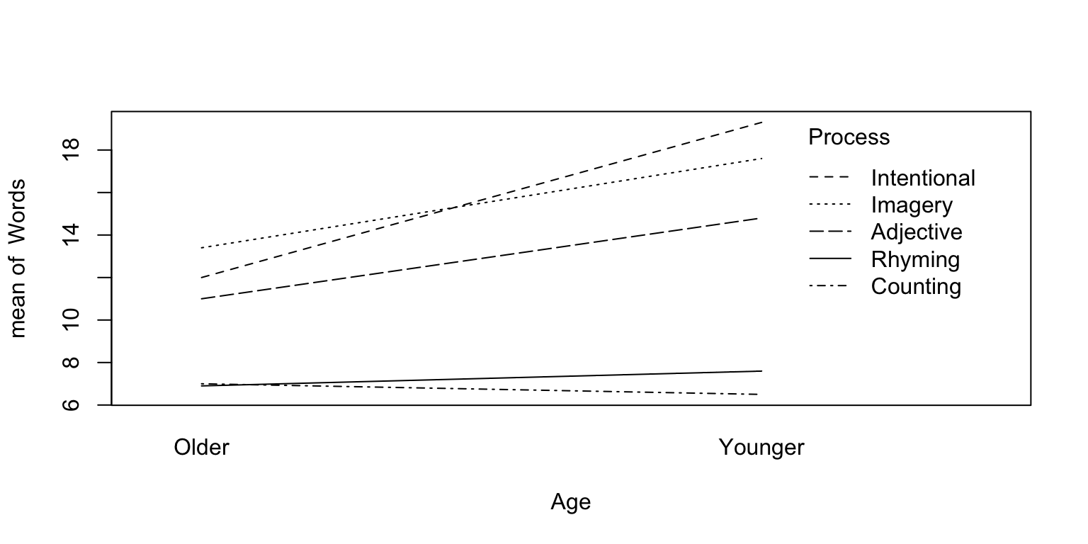
# while the interaction term is significant, but which level combinations are significant
# Estimate marginal means associated with 'Age' for each level of 'Process'.
fit3.emm <- emmeans(fit3, ~ Age | Process)
pairs(fit3.emm)
## Process = Adjective:
## contrast estimate SE df t.ratio p.value
## Older - Younger -3.8 1.27 90 -2.999 0.0035
##
## Process = Counting:
## contrast estimate SE df t.ratio p.value
## Older - Younger 0.5 1.27 90 0.395 0.6940
##
## Process = Imagery:
## contrast estimate SE df t.ratio p.value
## Older - Younger -4.2 1.27 90 -3.315 0.0013
##
## Process = Intentional:
## contrast estimate SE df t.ratio p.value
## Older - Younger -7.3 1.27 90 -5.762 <.0001
##
## Process = Rhyming:
## contrast estimate SE df t.ratio p.value
## Older - Younger -0.7 1.27 90 -0.553 0.5820Using the pairs function on an emmGrid object returns effect sizes and significance tests for each pairwise contrast.
The result shows, older subjects remember significantly fewer words than younger ones when using ‘Adjective, Imagery and Intentional’ processes but not the ‘Counting or Rhyming’ processes.
We could also contract different processes within each level of Age.
fit3.emm.2<-emmeans(fit3, ~ Process | Age)
pairs(fit3.emm.2)
## Age = Older:
## contrast estimate SE df t.ratio p.value
## Adjective - Counting 4.0 1.27 90 3.157 0.0180
## Adjective - Imagery -2.4 1.27 90 -1.894 0.3279
## Adjective - Intentional -1.0 1.27 90 -0.789 0.9331
## Adjective - Rhyming 4.1 1.27 90 3.236 0.0143
## Counting - Imagery -6.4 1.27 90 -5.052 <.0001
## Counting - Intentional -5.0 1.27 90 -3.947 0.0014
## Counting - Rhyming 0.1 1.27 90 0.079 1.0000
## Imagery - Intentional 1.4 1.27 90 1.105 0.8035
## Imagery - Rhyming 6.5 1.27 90 5.131 <.0001
## Intentional - Rhyming 5.1 1.27 90 4.025 0.0011
##
## Age = Younger:
## contrast estimate SE df t.ratio p.value
## Adjective - Counting 8.3 1.27 90 6.551 <.0001
## Adjective - Imagery -2.8 1.27 90 -2.210 0.1854
## Adjective - Intentional -4.5 1.27 90 -3.552 0.0054
## Adjective - Rhyming 7.2 1.27 90 5.683 <.0001
## Counting - Imagery -11.1 1.27 90 -8.761 <.0001
## Counting - Intentional -12.8 1.27 90 -10.103 <.0001
## Counting - Rhyming -1.1 1.27 90 -0.868 0.9077
## Imagery - Intentional -1.7 1.27 90 -1.342 0.6660
## Imagery - Rhyming 10.0 1.27 90 7.893 <.0001
## Intentional - Rhyming 11.7 1.27 90 9.235 <.0001
##
## P value adjustment: tukey method for comparing a family of 5 estimatescomparing models
- R-squared: a measure of Goodness of Fit.
- likelihood ratio test on two ‘nested’ models (
anovafunction). - AIC (Akaike’s Information Criterion), lowest AIC is the preferred model.
\(r^2\) or \(R^2\) Variance explaned
descriptive measure of association between Y and X (also termed coefficient of variation). the proportion of the total variation in Y that is explained by its linear relationship with X.
\[ R^2 = 1 - \frac{SS_{residual}}{SS_{total}} \]
# r-square indicates how much variation in the response variable is captured by the linear model
# as residual variation (ss.resid) means the varation part **not** captured by your model
# r-square = 1 - (ss.resid)/(ss.total)
summary(fit2)$r.squared
## [1] 0.6579191summary(fit3)$r.squared## [1] 0.7292516# calculate by hand
ss.resid = sum(residuals(fit2)**2)
total.var = sum((memory$Words-mean(memory$Words))**2)
1 - ss.resid/total.var## [1] 0.6579191ss.resid = sum(residuals(fit3)**2)
1 - ss.resid/total.var## [1] 0.7292516# perform an anova on two models to compare the fit.
# Note that one model must be a subset of the other model.
anova(fit2,fit3)## Analysis of Variance Table
##
## Model 1: Words ~ Age + Process
## Model 2: Words ~ Age * Process
## Res.Df RSS Df Sum of Sq F Pr(>F)
## 1 94 912.6
## 2 90 722.3 4 190.3 5.9279 0.0002793 ***
## ---
## Signif. codes: 0 '***' 0.001 '**' 0.01 '*' 0.05 '.' 0.1 ' ' 1AIC(fit2,fit3)## df AIC
## fit2 7 518.9005
## fit3 11 503.5147variance explained by each predictor
x<-Anova(fit3)
attributes(x)
## $names
## [1] "Sum Sq" "Df" "F value" "Pr(>F)"
##
## $class
## [1] "anova" "data.frame"
##
## $row.names
## [1] "Age" "Process" "Age:Process" "Residuals"
##
## $heading
## [1] "Anova Table (Type II tests)\n" "Response: Words"attr(x,'row.names')## [1] "Age" "Process" "Age:Process" "Residuals"x$`Sum Sq`## [1] 240.25 1514.94 190.30 722.30x$`Sum Sq`/sum(x$`Sum Sq`)## [1] 0.09005581 0.56786329 0.07133245 0.27074845diagnostics
- use Cook Statistics to detect influential observations
- normality of the residuals
influential point An influential point is one whose removal from the dataset would cause a large change in the fit. An influential point may or may not be an outlier and may or may not have large leverage but it will tend to have at least one of those two properties.
cook<-cooks.distance(fit3)
plot(cook,ylab='Cooks distances')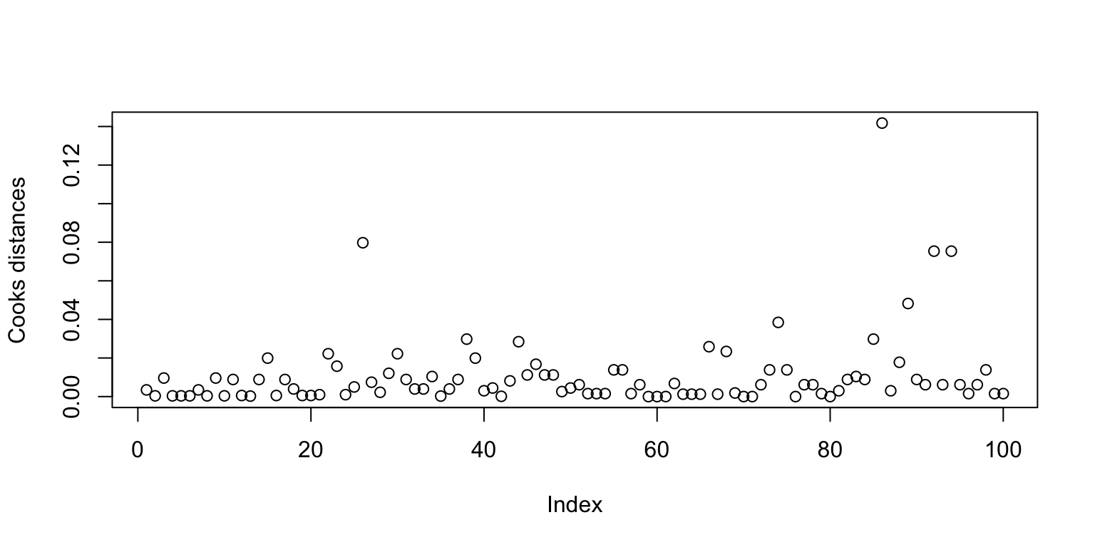
#Which ones are large? We now exclude the largest one and see how the fit changes:
gl <- lm(Words~Age*Process,data=memory,subset=(cook < max(cook)))
summary(gl)$r.squared
## [1] 0.755632summary(fit3)$r.squared## [1] 0.7292516residuals plot
par(mfrow=c(1,2))
# Residuals vs. fitted
residualPlot(fit3)
# QQ-plot of the residuals
invisible(qqPlot(fit3))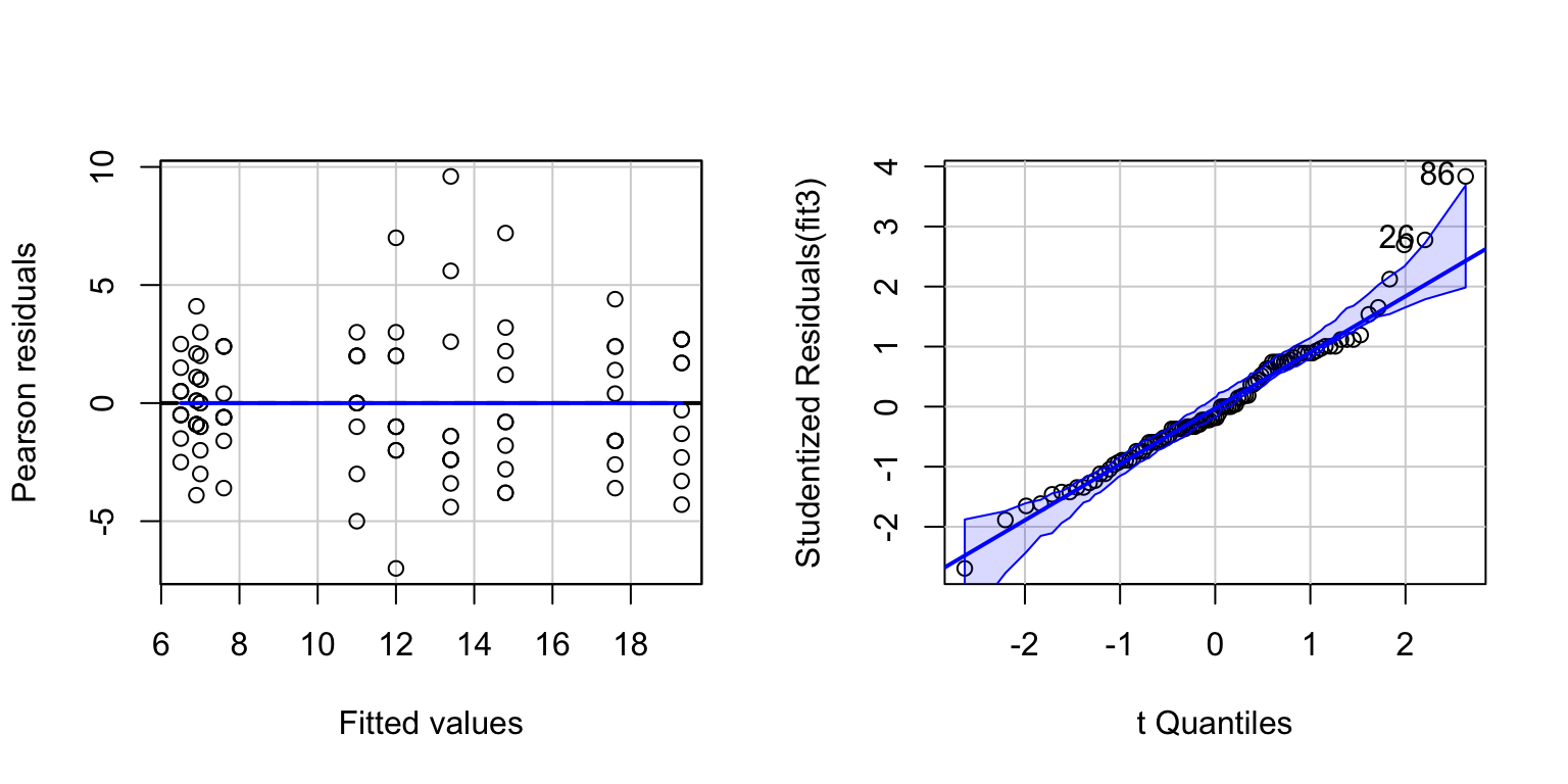
The QQ-plot shows some slight non-normality in the upper right. The non-normality probably stems from the fact that the Words variable is a ’count’ variable.
Check whether a log-transformation of Words makes the residuals closer to normally distributed.
par(mfrow=c(1,2))
gl<-lm(log10(Words)~Age*Process,data=memory)
residualPlot(gl)
invisible(qqPlot(gl))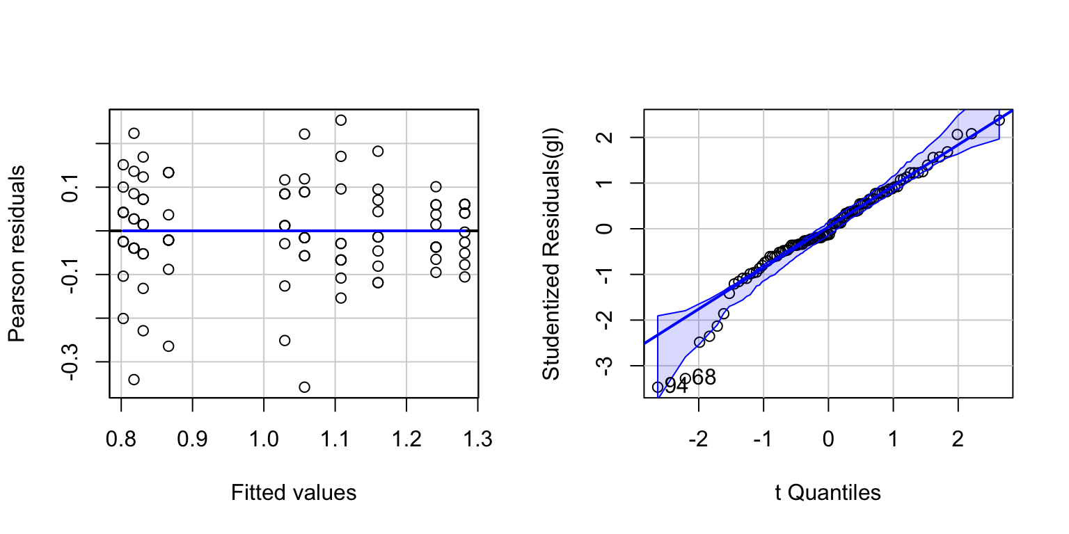
allom <- read.csv("allometry.csv")
fit4 <- lm(leafarea~diameter+height, data=allom)
# Basic diagnostic plots.
par(mfrow=c(1,2))
residualPlot(fit4)
invisible(qqPlot(fit4))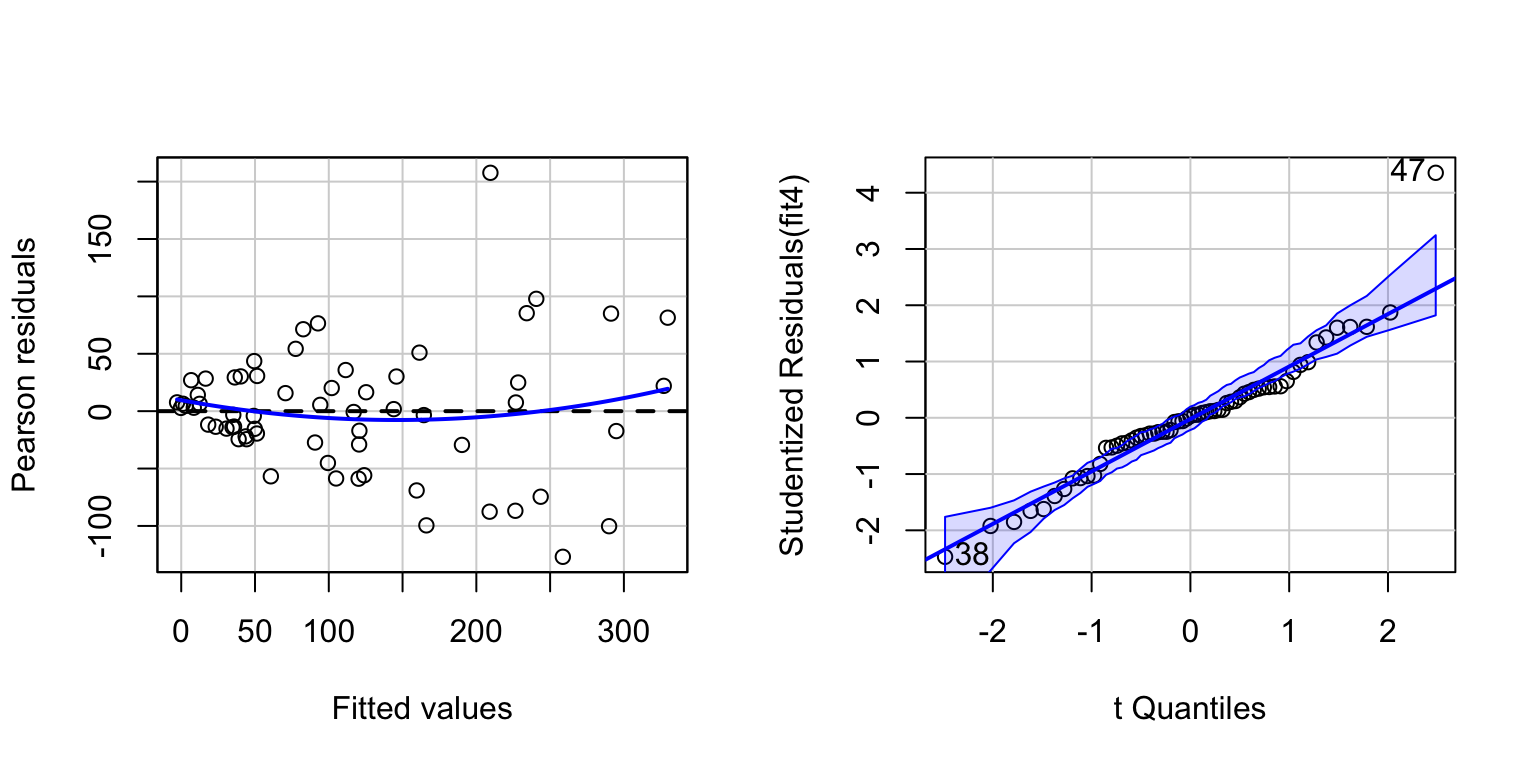
# For convenience, add log-transformed variables to the dataframe:
allom$logLA <- log10(allom$leafarea)
allom$logD <- log10(allom$diameter)
allom$logH <- log10(allom$height)
# Refit model, using log-transformed variables.
fit5 <- lm(logLA ~ logD + logH, data=allom)
# And diagnostic plots.
par(mfrow=c(1,2))
residualPlot(fit5)
invisible(qqPlot(fit5))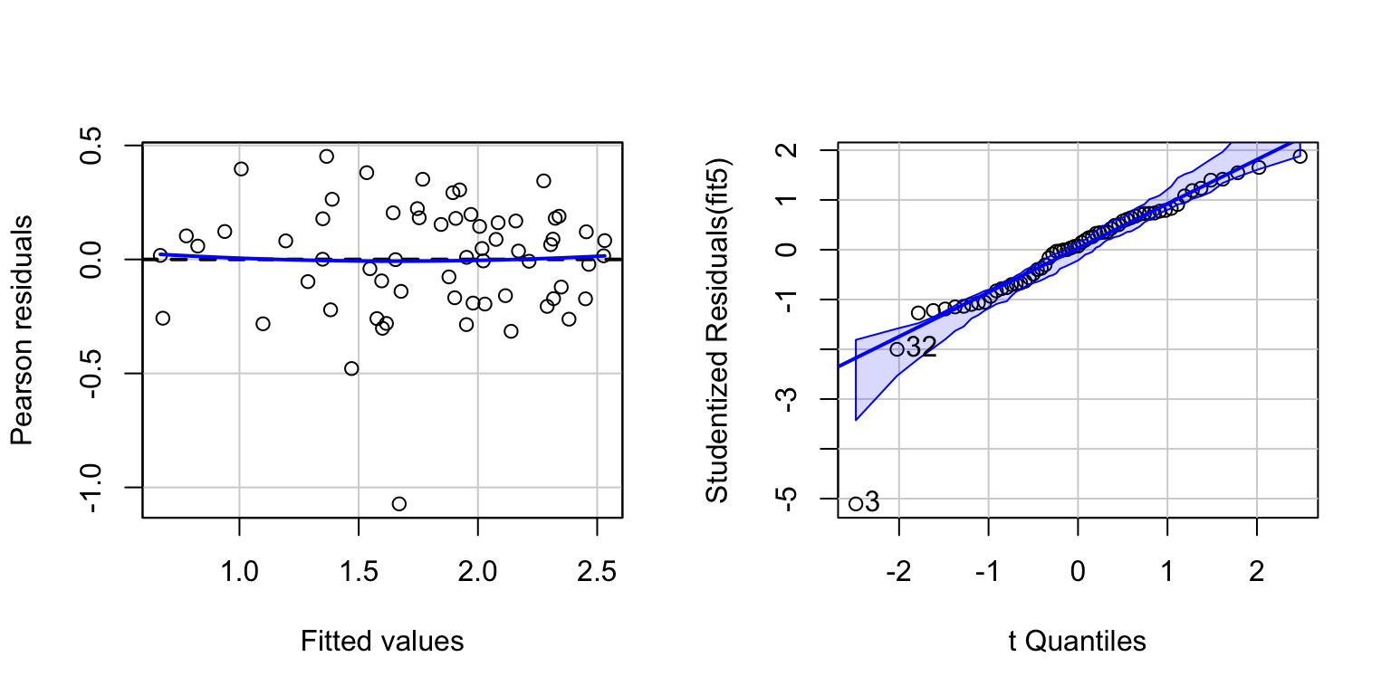
linear models with factors and continuous variables
# A linear model combining factors and continuous variables
fit7 <- lm(logLA ~ species + logD + logH, data=allom)
summary(fit7)
##
## Call:
## lm(formula = logLA ~ species + logD + logH, data = allom)
##
## Residuals:
## Min 1Q Median 3Q Max
## -1.10273 -0.09629 -0.00009 0.13811 0.38500
##
## Coefficients:
## Estimate Std. Error t value Pr(>|t|)
## (Intercept) -0.28002 0.14949 -1.873 0.06609 .
## speciesPIPO -0.29221 0.07299 -4.003 0.00018 ***
## speciesPSME -0.09095 0.07254 -1.254 0.21496
## logD 2.44336 0.27986 8.731 3.7e-12 ***
## logH -1.00967 0.29870 -3.380 0.00130 **
## ---
## Signif. codes: 0 '***' 0.001 '**' 0.01 '*' 0.05 '.' 0.1 ' ' 1
##
## Residual standard error: 0.2252 on 58 degrees of freedom
## Multiple R-squared: 0.839, Adjusted R-squared: 0.8279
## F-statistic: 75.54 on 4 and 58 DF, p-value: < 2.2e-16The summary of this fit shows that PIPO differs markedly from the base level species, in this case PIMO. However, PSME does not differ from PIMO. The linear effects in log diameter and log height remain significant.
An ANOVA table will tell us whether adding species improves the model overall (as a reminder, you need the car package loaded for this function).
Anova(fit7)## Anova Table (Type II tests)
##
## Response: logLA
## Sum Sq Df F value Pr(>F)
## species 0.8855 2 8.731 0.0004845 ***
## logD 3.8652 1 76.222 3.701e-12 ***
## logH 0.5794 1 11.426 0.0013009 **
## Residuals 2.9412 58
## ---
## Signif. codes: 0 '***' 0.001 '**' 0.01 '*' 0.05 '.' 0.1 ' ' 1Perhaps the slopes on log diameter (and other measures) vary by species. This is an example of an interaction between a factor and a continuous variable. We can fit this as:
# A linear model that includes an interaction between a factor and
# a continuous variable
# (species*logD is equivalent to species + logD + species:logD).
fit8 <- lm(logLA ~ species * logD + species * logH, data=allom)
summary(fit8)
##
## Call:
## lm(formula = logLA ~ species * logD + species * logH, data = allom)
##
## Residuals:
## Min 1Q Median 3Q Max
## -1.05543 -0.08806 -0.00750 0.11481 0.34124
##
## Coefficients:
## Estimate Std. Error t value Pr(>|t|)
## (Intercept) -0.3703 0.2534 -1.461 0.1498
## speciesPIPO -0.4074 0.3483 -1.169 0.2473
## speciesPSME 0.2249 0.3309 0.680 0.4997
## logD 1.3977 0.4956 2.820 0.0067 **
## logH 0.1610 0.5255 0.306 0.7606
## speciesPIPO:logD 1.5029 0.6499 2.313 0.0246 *
## speciesPSME:logD 1.7231 0.7185 2.398 0.0200 *
## speciesPIPO:logH -1.5238 0.6741 -2.261 0.0278 *
## speciesPSME:logH -2.0890 0.7898 -2.645 0.0107 *
## ---
## Signif. codes: 0 '***' 0.001 '**' 0.01 '*' 0.05 '.' 0.1 ' ' 1
##
## Residual standard error: 0.2155 on 54 degrees of freedom
## Multiple R-squared: 0.8626, Adjusted R-squared: 0.8423
## F-statistic: 42.39 on 8 and 54 DF, p-value: < 2.2e-16x<-model.matrix(fit8)
head(x)## (Intercept) speciesPIPO speciesPSME logD logH speciesPIPO:logD
## 1 1 0 1 1.737272 1.432007 0
## 2 1 0 1 1.541579 1.438067 0
## 3 1 0 1 1.396025 1.326950 0
## 4 1 0 1 1.457882 1.397245 0
## 5 1 0 1 1.541579 1.476976 0
## 6 1 0 1 1.578066 1.448242 0
## speciesPSME:logD speciesPIPO:logH speciesPSME:logH
## 1 1.737272 0 1.432007
## 2 1.541579 0 1.438067
## 3 1.396025 0 1.326950
## 4 1.457882 0 1.397245
## 5 1.541579 0 1.476976
## 6 1.578066 0 1.448242From the summary, the logD (log diameter) coefficient appears to be significant. In this example, this coefficient represents the slope for the base species, PIMO. (three levels for species: PIMO, PIPO, PSME)
Other terms, including speciesPIPO:logD, are also significant. This means that their slopes differ from that of the base species (PIMO).
We can also look at the Anova to decide whether adding these slope terms improved the model.
Anova(fit8)## Anova Table (Type II tests)
##
## Response: logLA
## Sum Sq Df F value Pr(>F)
## species 0.8855 2 9.5294 0.0002854 ***
## logD 3.9165 1 84.2945 1.286e-12 ***
## logH 0.6102 1 13.1325 0.0006425 ***
## species:logD 0.3382 2 3.6394 0.0329039 *
## species:logH 0.3752 2 4.0378 0.0232150 *
## Residuals 2.5089 54
## ---
## Signif. codes: 0 '***' 0.001 '**' 0.01 '*' 0.05 '.' 0.1 ' ' 1predicted effects
The coefficients in a linear model are usually contrasts (i.e. differences between factor levels), slopes or intercepts. While this is useful for comparisons of treatments, it is often more instructive to visualize the predictions at various combinations of factor levels.
library(effects)
# Fit linear model, main effects only
fit9 <- lm(Words ~ Age + Process, data=memory)
plot(allEffects(fit9))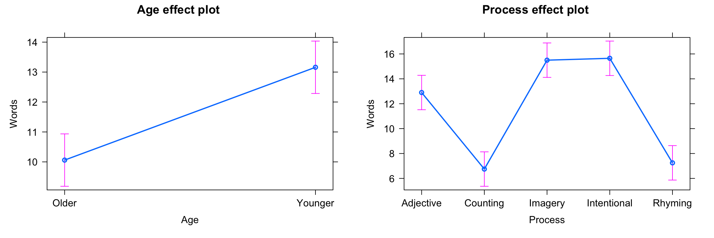
# compare the output when all all interactions
fit10 <- lm(Words ~ Age * Process, data=memory)
plot(allEffects(fit10))
Using predicted effects to make sense of model output
eucgas <- read.csv("eucface_gasexchange.csv")
eucgas$CO2=as.factor(eucgas$CO2)
par(mfrow=c(1,2))
palette(c("blue","red"))
with(eucgas, plot(Trmmol, Photo, pch=19, col=CO2))
legend("topleft", levels(eucgas$CO2), pch=19, col=palette())
boxplot(Photo ~ CO2, data=eucgas, col=palette(), ylab="Photo")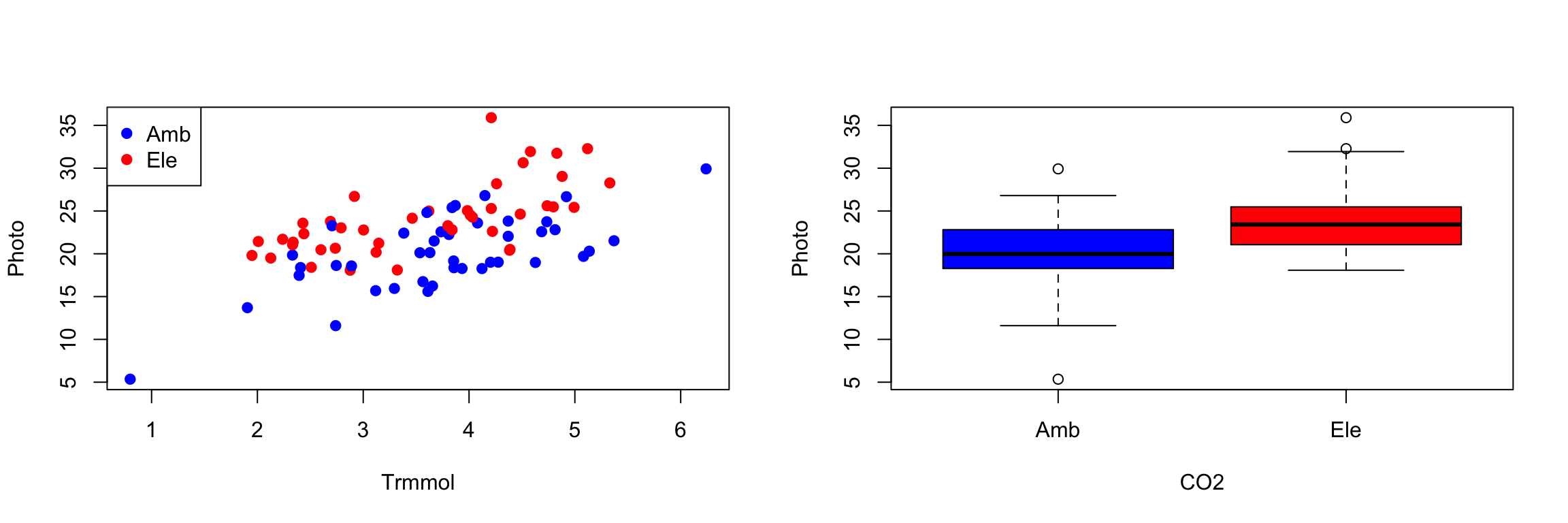
unique(eucgas$CO2)## [1] Ele Amb
## Levels: Amb Elesummary(eucgas$Trmmol)## Min. 1st Qu. Median Mean 3rd Qu. Max.
## 0.7978 2.8554 3.8049 3.6705 4.3732 6.2400summary(eucgas$Photo)## Min. 1st Qu. Median Mean 3rd Qu. Max.
## 5.352 19.128 22.146 22.117 24.682 35.900# A linear model with a continuous and a factor predictor, including the interaction.
lmfit <- lm(Photo ~ CO2*Trmmol, data=eucgas)
summary(lmfit)##
## Call:
## lm(formula = Photo ~ CO2 * Trmmol, data = eucgas)
##
## Residuals:
## Min 1Q Median 3Q Max
## -6.1387 -2.4643 -0.0251 2.0081 10.0718
##
## Coefficients:
## Estimate Std. Error t value Pr(>|t|)
## (Intercept) 9.1591 1.9365 4.730 9.52e-06 ***
## CO2Ele 5.0146 2.6956 1.860 0.0665 .
## Trmmol 2.9221 0.4974 5.875 9.25e-08 ***
## CO2Ele:Trmmol -0.1538 0.7091 -0.217 0.8288
## ---
## Signif. codes: 0 '***' 0.001 '**' 0.01 '*' 0.05 '.' 0.1 ' ' 1
##
## Residual standard error: 3.219 on 80 degrees of freedom
## Multiple R-squared: 0.5446, Adjusted R-squared: 0.5276
## F-statistic: 31.9 on 3 and 80 DF, p-value: 1.158e-13x<-model.matrix(lmfit)
head(x)## (Intercept) CO2Ele Trmmol CO2Ele:Trmmol
## 1 1 1 4.88 4.88
## 2 1 1 4.58 4.58
## 3 1 1 4.21 4.21
## 4 1 0 3.81 0.00
## 5 1 0 3.87 0.00
## 6 1 0 4.08 0.00head(eucgas[,c('CO2','Trmmol')])## CO2 Trmmol
## 1 Ele 4.88
## 2 Ele 4.58
## 3 Ele 4.21
## 4 Amb 3.81
## 5 Amb 3.87
## 6 Amb 4.08There are two levels for CO2: Amb and Ele
Look at the ’coefficients’ table in the summary statement. Four parameters are shown, they can be interpreted as,
- the intercept for ’Amb’: 9.159
- the difference in the intercept for ’Ele’, compared to ’Amb’: 5.014
- the slope for ’Amb’: 2.92
- the difference in the slope for ’Ele’, compared to ’Amb’: -0.153
# Significance of overall model terms (sequential anova)
anova(lmfit)
## Analysis of Variance Table
##
## Response: Photo
## Df Sum Sq Mean Sq F value Pr(>F)
## CO2 1 322.96 322.96 31.1659 3.142e-07 ***
## Trmmol 1 668.13 668.13 64.4758 7.074e-12 ***
## CO2:Trmmol 1 0.49 0.49 0.0471 0.8288
## Residuals 80 829.00 10.36
## ---
## Signif. codes: 0 '***' 0.001 '**' 0.01 '*' 0.05 '.' 0.1 ' ' 1It seems that neither the intercept or slope effect of CO2 is significant here, which is surprising.
Also confusing is the fact that the anova statement showed a clear significant effect of CO2, so what is going on here?
First recall that the sequential anova tests each term against a model that includes only the terms preceding it. So, since we added CO2 as the first predictor, its test in the anova is tested against a model that has no predictors.
This is similar in approach to simply performing a t-test on Photo vs. CO2 (which also shows a significant effect).
It is clearly a different test from those shown in the summary statement.
To understand the tests of the coefficients, we will plot predictions of the model, together with confi- dence intervals. We introduce the use of the predict function to estimate fitted values, and confidence intervals, from a fitted model.
# Set up a regular sequence of numbers, for which 'Photo' is to be predicted from
xval <- seq(0, max(eucgas$Trmmol), length=101)
# Two separate dataframes, one for each treatment/
amb_dfr <- data.frame(Trmmol=xval, CO2="Amb")
ele_dfr <- data.frame(Trmmol=xval, CO2="Ele")
# Predictions of the model using 'predict.lm'
# The first argument is the fitted model, the second argument a dataframe
# containing values for the predictor variables.
predamb <- as.data.frame(predict(lmfit, amb_dfr, interval="confidence"))
predele <- as.data.frame(predict(lmfit, ele_dfr, interval="confidence"))
head(amb_dfr)
## Trmmol CO2
## 1 0.0000 Amb
## 2 0.0624 Amb
## 3 0.1248 Amb
## 4 0.1872 Amb
## 5 0.2496 Amb
## 6 0.3120 Ambcolnames(model.matrix(lmfit))## [1] "(Intercept)" "CO2Ele" "Trmmol" "CO2Ele:Trmmol"head(predamb)## fit lwr upr
## 1 9.159077 5.305337 13.01282
## 2 9.341417 5.547339 13.13550
## 3 9.523758 5.789273 13.25824
## 4 9.706099 6.031136 13.38106
## 5 9.888439 6.272923 13.50396
## 6 10.070780 6.514631 13.62693# Plot. Set up the axis limits so that they start at 0, and go to the maximum.
palette(c("blue","red"))
with(eucgas, plot(Trmmol, Photo, pch=19, col=CO2,
xlim=c(0, max(Trmmol)),
ylim=c(0, max(Photo))))
# Add the lines; the fit and lower and upper confidence intervals.
with(predamb, {
lines(xval, fit, col="blue", lwd=2)
lines(xval, lwr, col="blue", lwd=1, lty=2)
lines(xval, upr, col="blue", lwd=1, lty=2)
})
with(predele, {
lines(xval, fit, col="red", lwd=2)
lines(xval, lwr, col="red", lwd=1, lty=2)
lines(xval, upr, col="red", lwd=1, lty=2)
})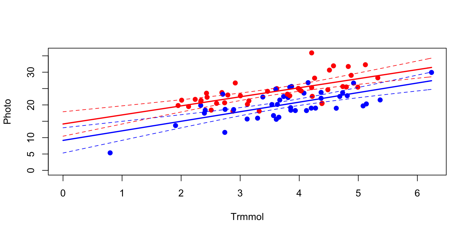
The confidence intervals for the regression lines overlap when Trmmol is zero - which is the comparison made in the summary statement for the intercept.
We now see why the intercept was not significant, but it says very little about the treatment difference in the range of the data. Perhaps it is more meaningful to test for treatment differences at a mean value of Trmmol. There are four ways to do this.
Centering the predictor
# Rescaled transpiration rate
# This is equivalent to Trmmol - mean(Trmmol)
eucgas$Trmmol_center <- scale(eucgas$Trmmol, center=TRUE, scale=FALSE)
# Refit using centered predictor
lmfit2 <- lm(Photo ~ Trmmol_center*CO2, data=eucgas)
summary(lmfit2)
##
## Call:
## lm(formula = Photo ~ Trmmol_center * CO2, data = eucgas)
##
## Residuals:
## Min 1Q Median 3Q Max
## -6.1387 -2.4643 -0.0251 2.0081 10.0718
##
## Coefficients:
## Estimate Std. Error t value Pr(>|t|)
## (Intercept) 19.8847 0.4989 39.861 < 2e-16 ***
## Trmmol_center 2.9221 0.4974 5.875 9.25e-08 ***
## CO2Ele 4.4500 0.7055 6.307 1.47e-08 ***
## Trmmol_center:CO2Ele -0.1538 0.7091 -0.217 0.829
## ---
## Signif. codes: 0 '***' 0.001 '**' 0.01 '*' 0.05 '.' 0.1 ' ' 1
##
## Residual standard error: 3.219 on 80 degrees of freedom
## Multiple R-squared: 0.5446, Adjusted R-squared: 0.5276
## F-statistic: 31.9 on 3 and 80 DF, p-value: 1.158e-13Using the effects package
Another way is to compute the CO2 effect at a mean value of Trmmol. This avoids having to refit the model with centered data, and is more flexible.
# The effects package calculates effects for a variable by averaging over all other
# terms in the model
library(effects)
Effect("CO2", lmfit)
##
## CO2 effect
## CO2
## Amb Ele
## 19.88469 24.33468# confidence intervals can be obtained via
summary(Effect("CO2", lmfit))##
## CO2 effect
## CO2
## Amb Ele
## 19.88469 24.33468
##
## Lower 95 Percent Confidence Limits
## CO2
## Amb Ele
## 18.89193 23.34178
##
## Upper 95 Percent Confidence Limits
## CO2
## Amb Ele
## 20.87745 25.32757#The effects package is quite flexible. For example, we can calculate the predicted effects at any speci- fied value of the predictors, like so (output not shown):
 # For example, what is the CO2 effect when Trmmol was 3?
summary(Effect("CO2", lmfit, given.values=c(Trmmol=3)))
##
## CO2 effect
## CO2
## Amb Ele
## 17.92545 22.47858
##
## Lower 95 Percent Confidence Limits
## CO2
## Amb Ele
## 16.68129 21.33201
##
## Upper 95 Percent Confidence Limits
## CO2
## Amb Ele
## 19.16961 23.62516Least-square means
The effect size while holding other predictors constant at their mean value is also known as the ’least- square mean’ (or even ’estimated marginal means’), and is implemented as such in the emmeans pack- age. It is a powerful package, also to make sense of models that are far more complex than the one in this example, as seen in section 7.2.1.1.
# For example, what is the CO2 effect when Trmmol was 3?
summary(Effect("CO2", lmfit, given.values=c(Trmmol=3)))##
## CO2 effect
## CO2
## Amb Ele
## 17.92545 22.47858
##
## Lower 95 Percent Confidence Limits
## CO2
## Amb Ele
## 16.68129 21.33201
##
## Upper 95 Percent Confidence Limits
## CO2
## Amb Ele
## 19.16961 23.62516library(emmeans)
summary(emmeans(lmfit, "CO2"))## CO2 emmean SE df lower.CL upper.CL
## Amb 19.9 0.499 80 18.9 20.9
## Ele 24.3 0.499 80 23.3 25.3
##
## Confidence level used: 0.95# emmeans warns that perhaps the results are misleading - this is true for more
# complex models but not a simple one as shown here.Using the predict function
Finally, we show that the effects can also be obtained via the use of predict, as we already saw in the code to produce Fig. 7.13.
# Predict fitted Photo at the mean of Trmmol, for both CO2 treatments
predict(lmfit, data.frame(Trmmol=mean(eucgas$Trmmol),
                          CO2=levels(eucgas$CO2)),
        interval="confidence")
## fit lwr upr
## 1 19.88469 18.89193 20.87745
## 2 24.33468 23.34178 25.32757Generalized Linear Models
So far we have looked at modelling a continuous response to one or more factor variables (ANOVA), one or more continuous variables (multiple regression), and combinations of factors and continuous variables.
We have also assumed that the predictors are normally distributed, and that, as a result, the response will be, too.
We used a log-transformation in one of the examples to meet this assumption.
In some cases, there is no obvious way to transform the response or predictors, and in other cases it is nearly impossible. Examples of difficult situations are when the response represents a count or when it is binary (i.e., has only two possible outcomes).
Generalized linear models (GLMs) extend linear models by allowing non-normally distributed errors. The basic idea is as follows.
Logistic regression is an example of a GLM, with a binomial distribution and the link-function log(u/(1-u) -> linear.predictor.
Another common GLM uses the Poisson distribution, in which case the most commonly used link- function is log. This is also called Poisson regression, and it is often used when the response represents counts of items.
Logistic Regression
# Read tab-delimited data
titanic <- read.table("titanic.txt", header=TRUE)
# Complete cases only (drops any row that has a missing value anywhere)
titanic <- titanic[complete.cases(titanic),]
# Construct a factor variable based on 'Survived'
titanic$Sex <- factor(titanic$Sex)
titanic$PClass <- factor(titanic$PClass)
titanic$Survived <- factor(ifelse(titanic$Survived==1, "yes", "no"))
# Look at a standard summary
summary(titanic)
## Name PClass Age Sex Survived
## Length:756 1st:226 Min. : 0.17 female:288 no :443
## Class :character 2nd:212 1st Qu.:21.00 male :468 yes:313
## Mode :character 3rd:318 Median :28.00
## Mean :30.40
## 3rd Qu.:39.00
## Max. :71.00par(mfrow=c(1,2), mgp=c(2,1,0))
with(titanic, plot(Sex, Survived, ylab="Survived", xlab="Sex"))
with(titanic, plot(PClass, Survived, ylab="Survived", xlab="Passenger class"))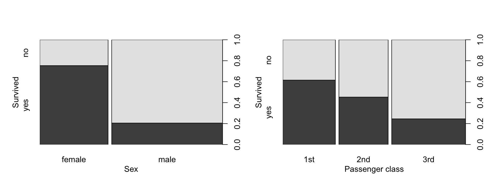
In logistic regression we model the probability of the “1” response (in this case the probability of sur- vival). Since probabilities are between 0 and 1, we use a logistic transform of the linear predictor, where the linear predictor is of the form we would like to use in the linear models above.
# Fit a logistic regression
fit11 <- glm(Survived~Age+Sex+PClass, data=titanic, family=binomial)
summary(fit11)
##
## Call:
## glm(formula = Survived ~ Age + Sex + PClass, family = binomial,
## data = titanic)
##
## Deviance Residuals:
## Min 1Q Median 3Q Max
## -2.7226 -0.7065 -0.3917 0.6495 2.5289
##
## Coefficients:
## Estimate Std. Error z value Pr(>|z|)
## (Intercept) 3.759662 0.397567 9.457 < 2e-16 ***
## Age -0.039177 0.007616 -5.144 2.69e-07 ***
## Sexmale -2.631357 0.201505 -13.058 < 2e-16 ***
## PClass2nd -1.291962 0.260076 -4.968 6.78e-07 ***
## PClass3rd -2.521419 0.276657 -9.114 < 2e-16 ***
## ---
## Signif. codes: 0 '***' 0.001 '**' 0.01 '*' 0.05 '.' 0.1 ' ' 1
##
## (Dispersion parameter for binomial family taken to be 1)
##
## Null deviance: 1025.57 on 755 degrees of freedom
## Residual deviance: 695.14 on 751 degrees of freedom
## AIC: 705.14
##
## Number of Fisher Scoring iterations: 5 # The 'type' argument is used to back-transform the probability
# (Try this plot without that argument for comparison)
plot(allEffects(fit11), type="response")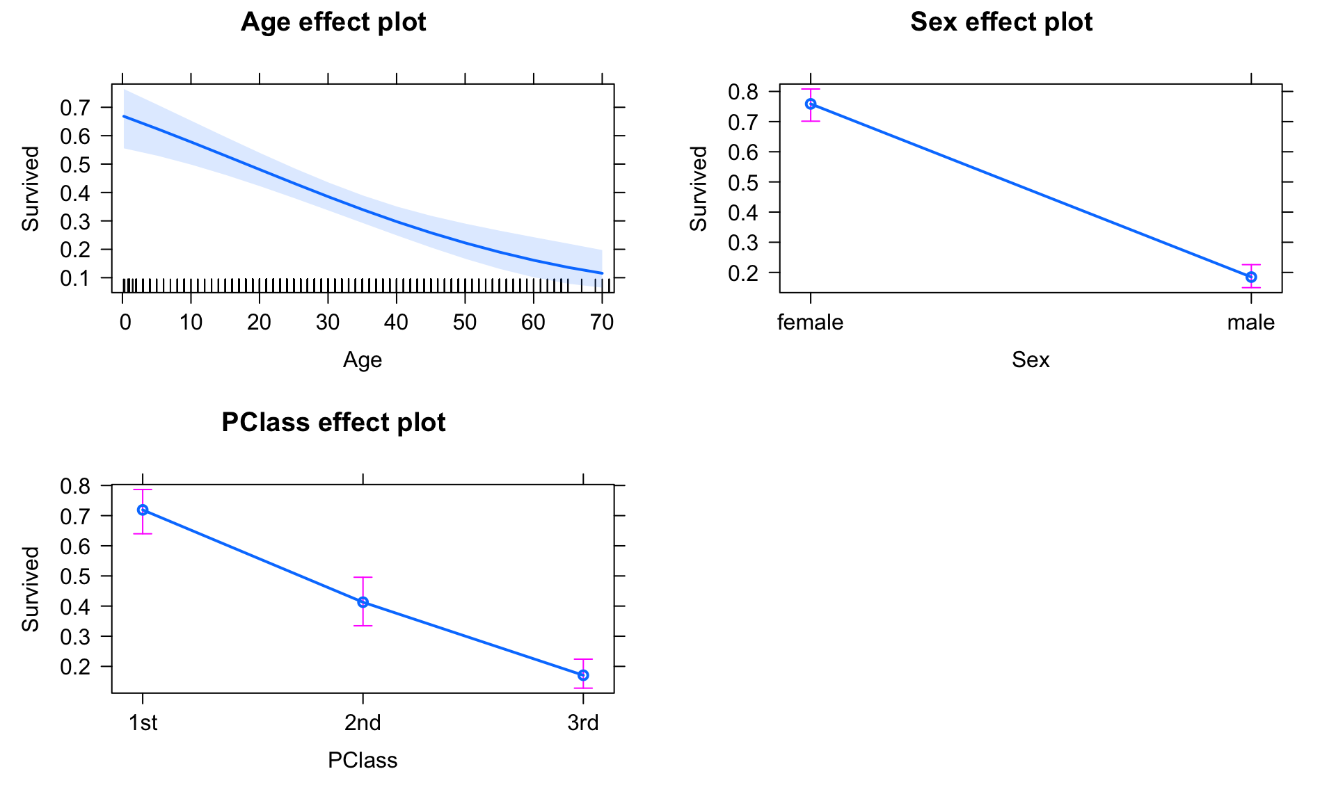
Poisson regression
# Fit a generalized linear model
fit13 <- glm(Words~Age*Process, data=memory, family=poisson)
summary(fit13)
##
## Call:
## glm(formula = Words ~ Age * Process, family = poisson, data = memory)
##
## Deviance Residuals:
## Min 1Q Median 3Q Max
## -2.2903 -0.4920 -0.1987 0.5623 2.3772
##
## Coefficients:
## Estimate Std. Error z value Pr(>|z|)
## (Intercept) 2.39790 0.09535 25.149 < 2e-16 ***
## AgeYounger 0.29673 0.12589 2.357 0.01842 *
## ProcessCounting -0.45199 0.15289 -2.956 0.00311 **
## ProcessImagery 0.19736 0.12866 1.534 0.12504
## ProcessIntentional 0.08701 0.13200 0.659 0.50978
## ProcessRhyming -0.46637 0.15357 -3.037 0.00239 **
## AgeYounger:ProcessCounting -0.37084 0.21335 -1.738 0.08218 .
## AgeYounger:ProcessImagery -0.02409 0.17027 -0.141 0.88750
## AgeYounger:ProcessIntentional 0.17847 0.17135 1.042 0.29764
## AgeYounger:ProcessRhyming -0.20011 0.20856 -0.959 0.33733
## ---
## Signif. codes: 0 '***' 0.001 '**' 0.01 '*' 0.05 '.' 0.1 ' ' 1
##
## (Dispersion parameter for poisson family taken to be 1)
##
## Null deviance: 227.503 on 99 degrees of freedom
## Residual deviance: 60.994 on 90 degrees of freedom
## AIC: 501.32
##
## Number of Fisher Scoring iterations: 4# Look at an ANOVA of the fitted model, and provide likelihood-ratio tests.
Anova(fit13)## Analysis of Deviance Table (Type II tests)
##
## Response: Words
## LR Chisq Df Pr(>Chisq)
## Age 20.755 1 5.219e-06 ***
## Process 137.477 4 < 2.2e-16 ***
## Age:Process 8.277 4 0.08196 .
## ---
## Signif. codes: 0 '***' 0.001 '**' 0.01 '*' 0.05 '.' 0.1 ' ' 1# Plot fitted effects
plot(allEffects(fit13))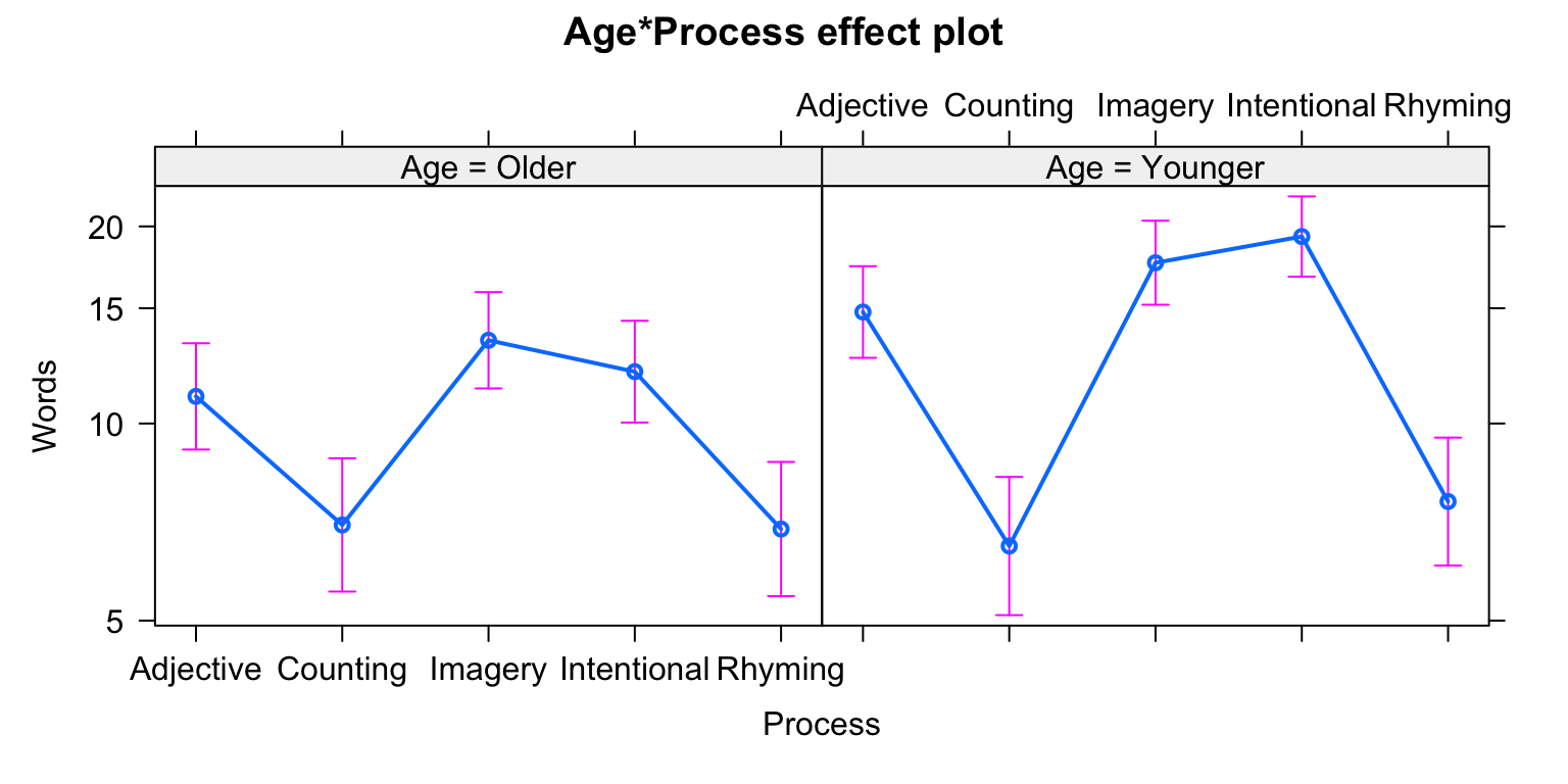
Note that in example above we use the anova function with the option test=“LRT”, which allows us to perform a Likelihood Ratio Test (LRT). This is appropriate for GLMs because the usual F-tests may not be inaccurate when the distribution is not normal.